Chapter 1 Introduction To Statistics

Outline:

Introduction

Revision and Topics Assumed - Exploratory Data Analysis (EDA) and Probability (separate document)

Using the R computer software:

Accessing R

Using R within R Studio.

Creating A Basic R Script (numerical summaries, plots, tables)

Accompanying Workshop (done in week 2):

Using R - Using RStudio; Creating a project; writing and saving commands;

Entering data; viewing data;

Basic EDA - summary(), boxplot(), table(), histogram()

Workshop for Week 1

Nil

Project Requirements for Week 1

Nil

Things for you to Check in Week 1

Ensure you have enrolled in a workshop;

If you intend to use University computers ensure your computing account is active and accessible;

Read the lecture notes for week 1 (these notes).

Try out R (eg go to the R section at the end of these notes and try to type and run the code there).

1.1 Statistics

Why Statistics? (What is Statistics?)
why do I need to use statistics?
what is a statistical test?
what do the results of a statistical test mean?
what is statistical significance?
how does probability fit in?

Statistical Inference requires assumptions about the data being analysed.

Lack of awareness and/or concern for assumptions leads to “misuse”:

You can prove anything with statistics.

There are three types of lies; lies, damned lies and statistics.

Statistics is concerned with scientific methods for collecting, organizing, summarizing, presenting and analyzing data as well as with drawing valid conclusions and making reasonable decisions on the basis of such analysis.

We can no more escape data than we can avoid the use of words. With data comes variation. Statistics is a tool to understand variation.

1.2 Individuals and Variables

Individuals: the objects described by the data – may be people, but not necessarily. Need clear definition of what individuals the data describe and how many of them there are in the data.

Variable: A measurement made on an individual – a characteristic of an individual.

Example: A researcher randomly selects 100 trees from Toohey forest and measures their height (H) and circumference at chest height (CCH). In this example the individuals are trees in Toohey forest (there are 100 individuals in this study). There are two variables: H and CCH.

1.3 Random Variables and Variation

A random variable is a variable whose value may change depending on chance.

The name of a random variable will often be symbolised by an upper case letter, e.g.: $X, Q, P, S, Y, Z$.

A particular value (or realisation) of a random variable is called a variate, and is often symbolised by a lower case letter, e.g.: $x, q, p, s, y, z$.

1.4 Statistical Populations

In statistics the term population refers to the totality of the data to which reference is to be made. It is critically dependent on the measurement being made and the question being asked.

There may be more than one population within the same problem. Some examples of different types of populations are:

finite versus infinite
real versus conceptual
univariate versus multivariate
quantitative versus qualitative
discrete versus continuous

A statistical population can be described using the distribution of its measurements or in terms of the probabilities of the values of a random variable.

1.5 Uncertainty, Error and Variability

The historical development of statistical theory began with the theory of errors. Note the following entry from the Encyclopedia Britannica:

A physical occurrence can seldom if ever be reproduced exactly. In particular the carefully staged physical occurrences known as scientific experiments are never capable of exact repetition. For example the yield of a product from a chemical reaction may vary quite considerably from one occasion to another due to slight differences of conditions such as temperature, pressure, concentration and agitation rate. Other errors will be introduced because of the impossibility of obtaining an entirely representative sample of the product for analysis. Finally, no method of chemical analysis of the sampled material will be exactly reproducible. The application of probability theory to the treatment of these various discrepancies is called the theory of errors.

Error $\neq$ uncertainty. Both are present to some extent in any scientific research.

Error: experimental error AND natural variability

Uncertainty: sampling AND lack of knowledge

1.6 Research Studies & Scientific Investigations

There are two main categories of scientific investigations:

Exploratory - fact finding, often with no specific hypothesis in mind.

Controlled Experimentation - investigations which begin with specific hypothesis. In this latter category there are 2 main types of study:

Observational Study – take measurements of something happening without control.
Experiment – manipulative, do something to observe a response – control.

1.7 Probability

A vital tool in statistics. See the assumed knowledge notes for a basic introduction.

The Study of Randomness – probability theory - describes random behaviour. Note that random does not mean haphazard.

There are numerous schools of thought when it comes to defining what ‘probability’ means. One definition states:

… ‘empirical probability’ of an event is taken to be the ‘relative frequency’ of occurrence of the event when the number of observations is very large. The probability itself is the ‘limit’ of the relative frequency as the number of observations increases indefinitely.

Note there are different conceptualizations of probability: empirical, theoretical, subjective – We will assume the empirical approach in this course.

1.8 Statistical Inference

There are two main phases in any statistical analysis:

Exploratory Data Analysis – See separate assumed knowledge notes.

Statistical Inference – See below.

One can undertake exploratory data analysis without progressing to inference. Conversely, in practice any inferential process should always be preceded by an exploration of the data in order to understand the data more fully.

1.8.1 Introduction to Statistical Inference

Research is carried out to find out about generalities. Advances in human knowledge generally rely on being able to state that something will happen in most cases. BUT, we rarely have information for all cases.

Population and Sample: Note that population does not necessarily refer to people.

Population: the totality of individual observations about which inferences are to be made

Sample: a subset of the population. The part of the population that we actually examine in order to gather information.

Why Sample? - (a) Cost: Resources available for study limited, as are time and effort. - (b) Utility: In some cases items may be destroyed in the process of sampling. - (c) Accessibility: Impracticable or even impossible to measure an entire population.

Example of inference in every day life:

On a cold morning, should we wear warm clothes for the day ahead, or will it warm up during the day?

Statistical Inference: a set of procedures used in making appropriate conclusions and generalisations about a whole (the population), based on a limited number of observations (the sample).

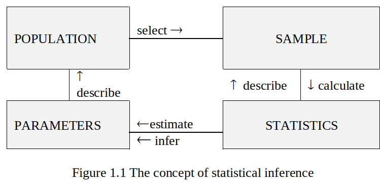
In general: Statistics are calculated from a sample and describe that sample.

Parameters are inferred from the calculated statistics.
Parameters are used to describe the population.
Therefore, statistics can be used to infer things about a population.

If all the population values were available, the population parameters would simply be found by calculating them from the values available. This is what the Australian Bureau of Statistics attempts to do when it conducts the census.

A population parameter has no error. It is an exact value which never changes (assumption).

Sample statistics depend on the particular sample of data selected and thus may vary in value; they represent a random variable and as such have variation. A statistic should never be quoted without some estimate of its variation; usually this is provided as a standard error of the statistic.

1.8.2 Estimation and Hypothesis Testing

There are two basic branches of statistical inference: estimation and hypothesis testing.

Both make use of statistics calculated from sample data, and each has a specific role to play in statistical inference. The choice of which to use depends on the question being asked.

What is the value of something? - This would entail estimation.

Versus

Are two things the same? – This would entail hypothesis testing.

The basic principles of estimation & hypothesis testing are the same for ALL types of parameters and statistics. However, the details may change. For example:

How to calculate the test statistic & estimate the standard error, and what probability distribution to use, are both important considerations in any inferential procedure and have situation-specific nswers (which we will deal with later).

BUT

If you have a basic understanding of the concepts you will easily cope with most situations.

1.9 Using The R Software - Week 1.

1.9.1 Accessing R in the common use computer labs

If you wish to install your own copy of R at home or on your laptop, both R and RStudio are free to download and use. Please see the information in Other Resources on the L@G site.
R and RStudio are installed on all common use computers across the University. Note that nothing can be saved on Uni computers, so make sure you save all work to a project on your USB stick (or similar) if using Uni computers, or else you will lose all your work when you log off and shut down. Tutors will help you with this in workshops.

1.9.2 Using R Within RStudio

There are four main windows in RStudio:

Script - where you write the programs and code.
Console - where the code from the script is run: output and errors appear here also.
Environment - Data, variables, functions etc are shown here, as well as a tab that records the “history” of your analysis.
Plot/Help - Any graphs you create, as well as the online help, plus a file explorer, are shown here (using tabs).

The four windows usually appear together as a split screen. Note that when you first open RStudio the script window may not appear – see the notes on using RStudio for creating projects for details on how to open a new R script.

1.9.3 Getting Help

R has an excellent online ‘help’ facility within the once you get used to it. Alternatives include searching the internet for R code help but just be aware, as with all of the internet, that there are good and bad sources on the web. If in doubt ask your lecturer or tutor.

The online help system in R is accessed in the help tab in the bottom right window of RStudio. You can read the manuals if you wish, or else you can search for specific functions in R to learn the syntax and what arguments the function requires. See the Rintro notes and lectures for some examples of how to use the help system within R.

Invaluable Help

As you move through the course you should try the code given to you (and obviously write your own as well!) and document what each step in the code does. R allows you to put comments in the script files, and this is very useful to give you reminders about what each piece of code does. Save these R scripts on your computer (perhaps in their own project areas – see the notes on creating and using R projects in RStudio).

You will find these R script files, containing code demonstrated in lectures, in each week’s lecture notes folder. You should download, save, and try running the code in these files. They often have a lot of comments in them, and you should feel free to add your own as well to help you understand what is happening from your own perspective. You will be expected and encouraged to create your own script files in workshops to help you do certain questions and analyses. Save these in some sort of systematic way, and comment them extensively so that when you look at them again for revision in week 12 (or later in your career when you need to analyze some data) it is not a complete mystery to you!

1.9.4 Creating an R script/program

Some Initial Notes

R is case sensitive – bla is different to Bla in R’s computer brain.
Use of a hash at start of a line indicates R is not to read that line – this is ideal for putting comments and reminders in your code.
R uses “object oriented” programming – everything in R is, or can be made into, an “object”. For our purposes this basically means we can and should give everything we do a name using the assignment operator. For example x <- rnorm(1000). There is now an object called x that contains 1000 random numbers from a normal distribution. Next time we need those numbers, we simply use x. The kinds of names we should use will be discussed in lectures.
We write our code in the script window in RStudio, and we run it by putting the cursor on the line of code we wish to run and clicking the run button.

A Inputting DATA

Most statistical analyses start with data, and so most analyses in R begin by entering, or reading in, data. R has many functions to read in data (mostly related to the kind of file the data is originally stored in, like Excel or text files). Data should be given a name so that it is easily available after we input it. For example:

rain.dat <- a.function.that.reads.in.data(“from an excel file”)

In this example we are using a function (I made its name up – we’ll see the correct function name shortly) to read in data from a file (I’ve made up a strange name for the file too…!) and I’ve put the result into an object that I’ve called rain.dat. Now there is a data set in R called rain.dat, and if I remember to save each time I quit R, rain.dat will be there when I next open R, forever, or until I choose to delete it. I never have to read the data into R again after this initial data input.

So let’s look at a proper example. The table below gives the rainfall over four seasons in five different districts.

District	Season
	Winter	Spring	Summer	Autumn
1	23	440	800	80
2	250	500	1180	200
3	120	400	420	430
4	10	20	30	5
5	60	200	250	120

Here there are three variables, district, season and rainfall – each measurement has 3 parts to it - trivariate. Note that the data is in a compressed form – typically each variable should have its own column, like this:

District	Season	Rainfall
1	Winter	23
1	Spring	440
1	Summer	800
1	Autumn	80
2	Winter	250
2	Spring	500
2	Summer	1180
2	Autumn	200
…	…	…

An Excel file with the data in this form can be found in the lecture notes folder for week 1.

There are two ways to import this data into R. The first is to use the Import Dataset menu in the Environment window in RStudio. This will be shown in the lecture.

The second way is a useful shortcut when you have small to moderate sized data (say less than a few thousand rows of data). R allows you to copy the data using your mouse/keyboard, and then enter it using the following code:

rainfall <- read.table(“clipboard”, header = T) #On Windows

rainfall <- read.table(pipe(“pbpaste”), header = T) #On MacOSX

This will also be demonstrated in lectures.

B Accessing, Exploring, Graphing and Analysing

Once the data set has been entered various analyses can proceed. R uses functions to do analyses, graphs and summaries.

1. Printing/Viewing: typing the name of the variable/dataset will print it in the command window:

rainfall <- read.csv("rainfall.csv")

rainfall

##    District Season Rainfall
## 1         1 Winter       23
## 2         1 Spring      440
## 3         1 Summer      800
## 4         1 Autumn       80
## 5         2 Winter      250
## 6         2 Spring      500
## 7         2 Summer     1180
## 8         2 Autumn      200
## 9         3 Winter      120
## 10        3 Spring      400
## 11        3 Summer      420
## 12        3 Autumn      430
## 13        4 Winter       10
## 14        4 Spring       20
## 15        4 Summer       30
## 16        4 Autumn        5
## 17        5 Winter       60
## 18        5 Spring      200
## 19        5 Summer      250
## 20        5 Autumn      120

Accessing variables within a dataset is achieved by prepending the name of the variable to the name of the dataset followed by a dollar sign like this: datasetname$variablename:

rainfall$Season

##  [1] "Winter" "Spring" "Summer" "Autumn" "Winter" "Spring" "Summer" "Autumn"
##  [9] "Winter" "Spring" "Summer" "Autumn" "Winter" "Spring" "Summer" "Autumn"
## [17] "Winter" "Spring" "Summer" "Autumn"

rainfall$Rainfall

##  [1]   23  440  800   80  250  500 1180  200  120  400  420  430   10   20   30
## [16]    5   60  200  250  120

rainfall$District

##  [1] 1 1 1 1 2 2 2 2 3 3 3 3 4 4 4 4 5 5 5 5

2. Basic EDA – numerical summary of data using summary() and table() functions:

For the rainfall example:

summary(rainfall)

##     District    Season             Rainfall     
##  Min.   :1   Length:20          Min.   :   5.0  
##  1st Qu.:2   Class :character   1st Qu.:  52.5  
##  Median :3   Mode  :character   Median : 200.0  
##  Mean   :3                      Mean   : 276.9  
##  3rd Qu.:4                      3rd Qu.: 422.5  
##  Max.   :5                      Max.   :1180.0

summary(rainfall$Rainfall)

##    Min. 1st Qu.  Median    Mean 3rd Qu.    Max. 
##     5.0    52.5   200.0   276.9   422.5  1180.0

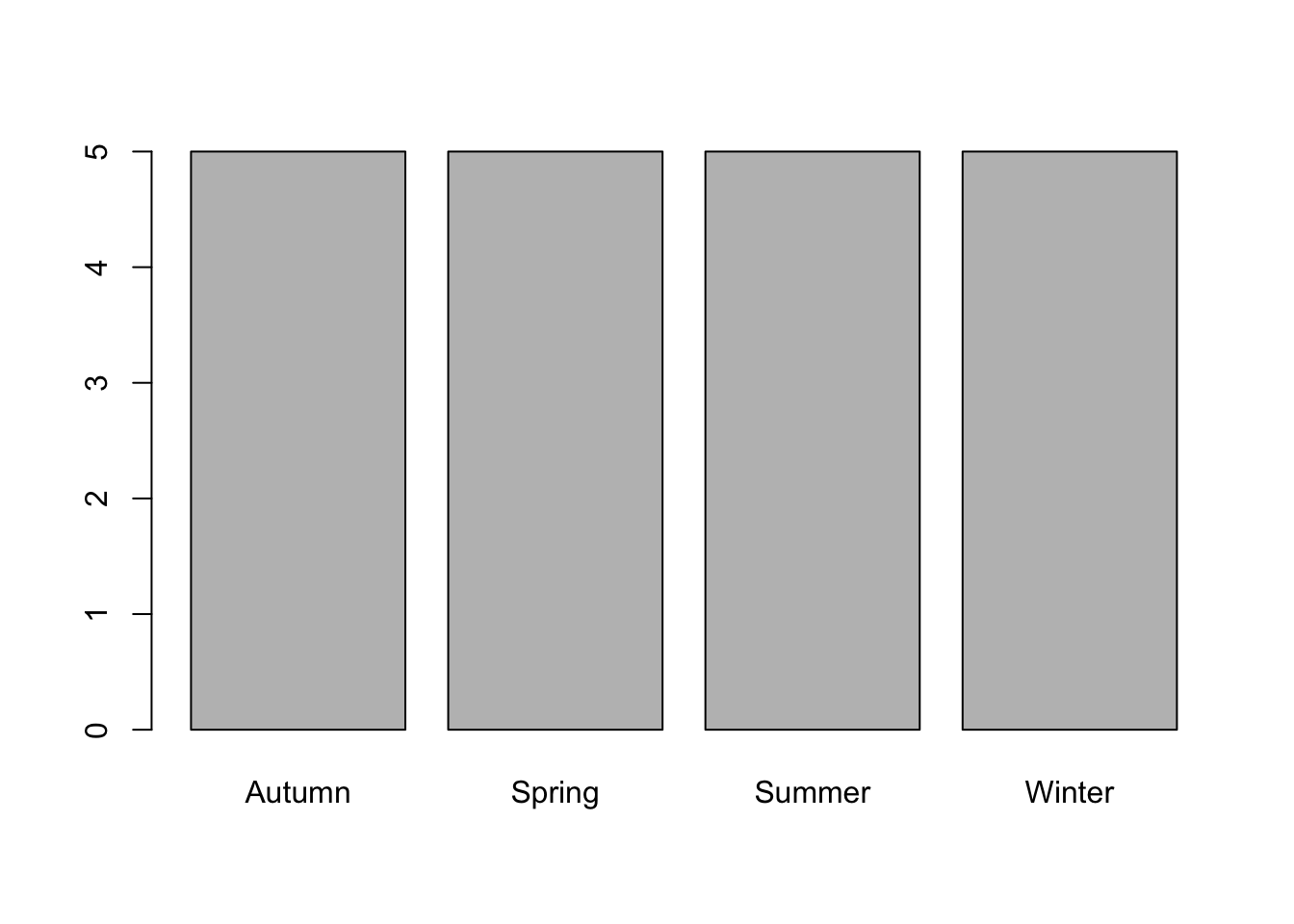
table(rainfall$Season) #for categorical variables

## 
## Autumn Spring Summer Winter 
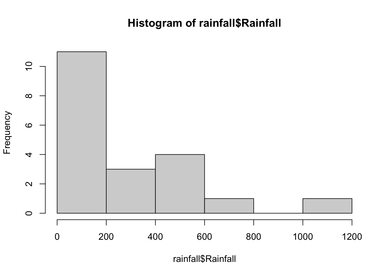
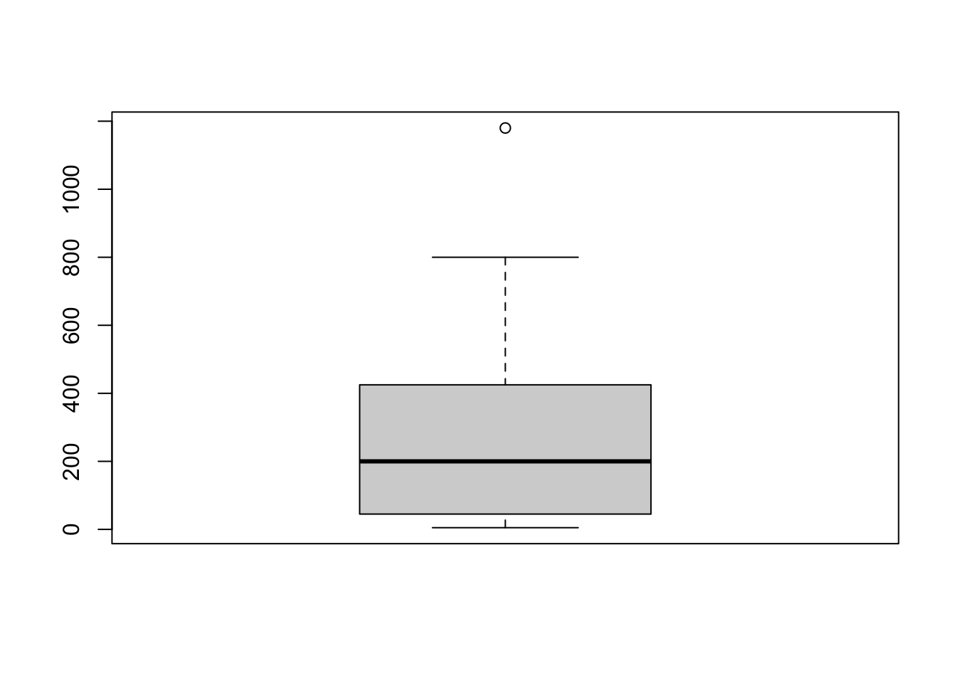
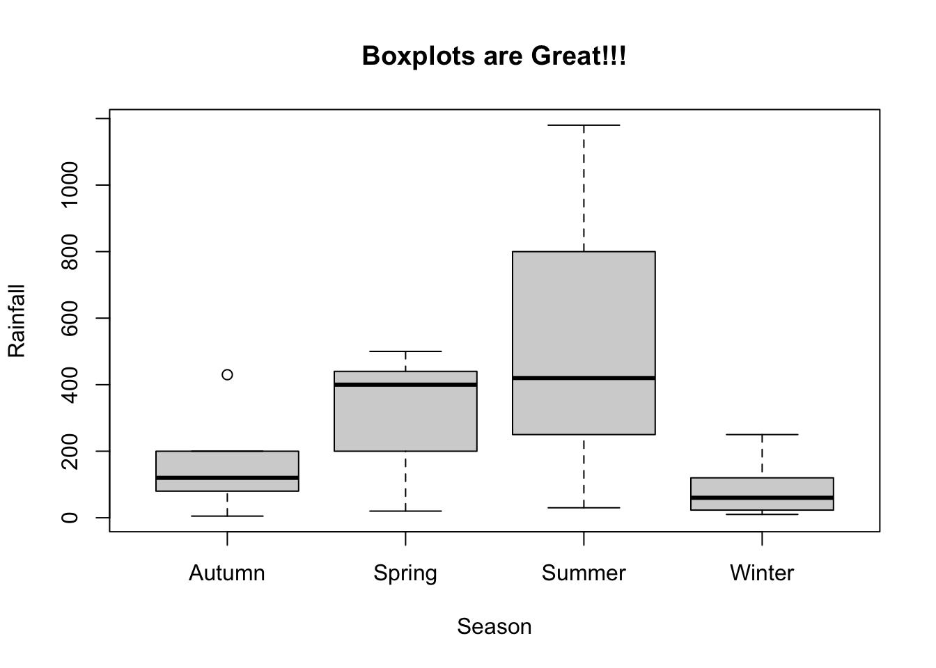
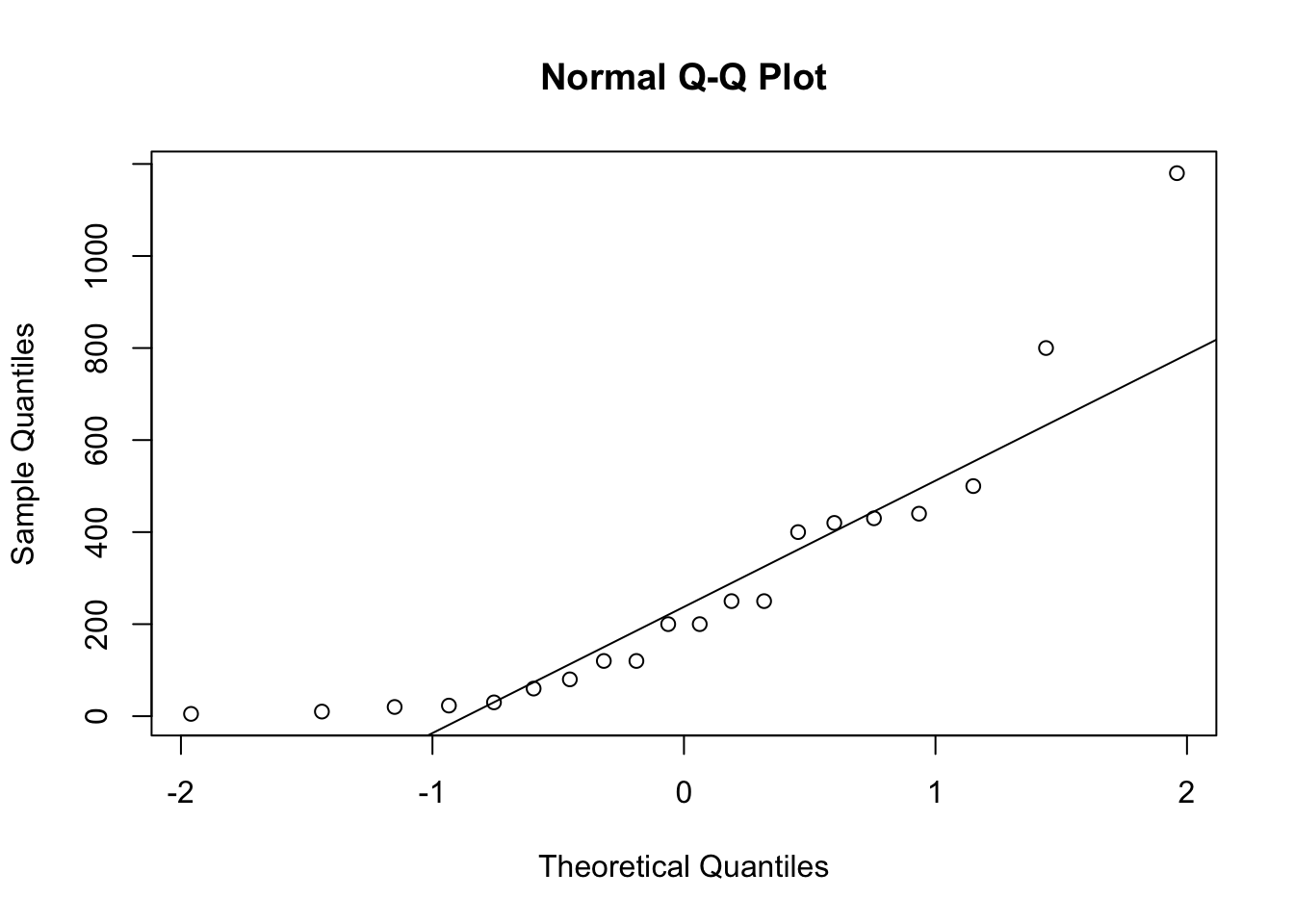
##      5      5      5      5

3. Graphs - Histograms, Boxplots, Quantile-Quantile (QQ) plots, Barplots: