Module 2 Analysis
This section will go through the main analysis pipeline and explain each element you need to generate your own results, and interpret them.
2.1 Dataset options
2.1.1 Upload data
To get started quickly, you may choose to explore a public demo datasets. Click on “Use demo data” to begin using the dataset for the analysis, or click “Download” to save the dataset locally. The latter option can be useful if you want to inspect the dataset as a spreadsheet and try to replicate the format with your own dataset.
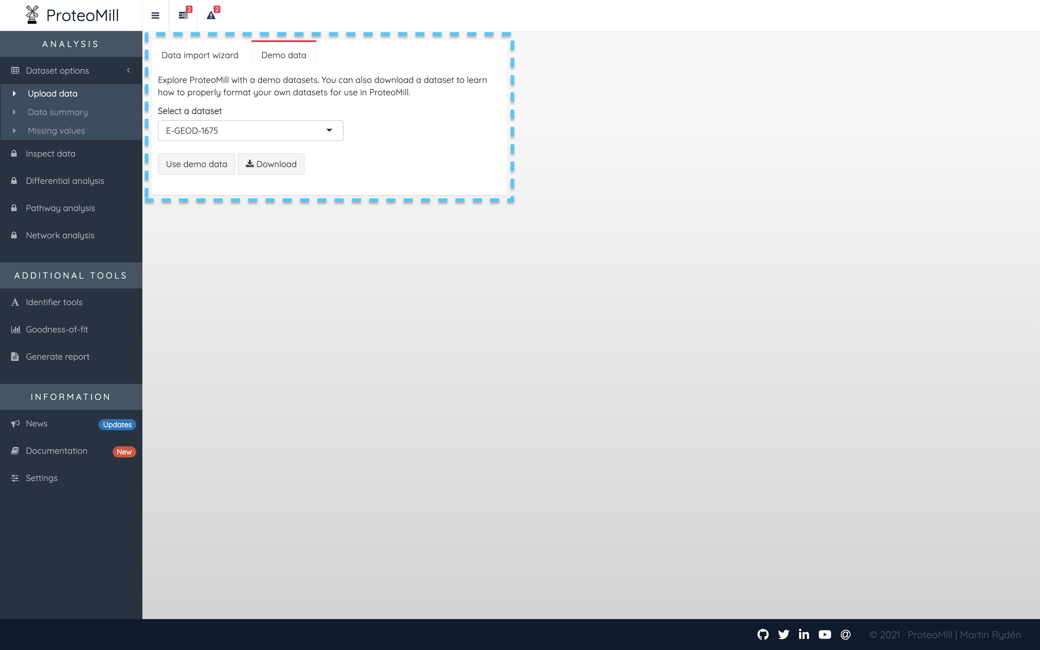
Figure 2.1: Demo dataset
To upload your own dataset, click on “Data import wizard”. Select organism in the list under “Sample information”. If your species is not available, you may still select “Other” but please note that functionality that requires annotation data (pathway and network analysis) will not be available. We are continuously adding support for more organisms.
Only if your data is already log₂-transformed, uncheck the box “Log₂-transform data”.
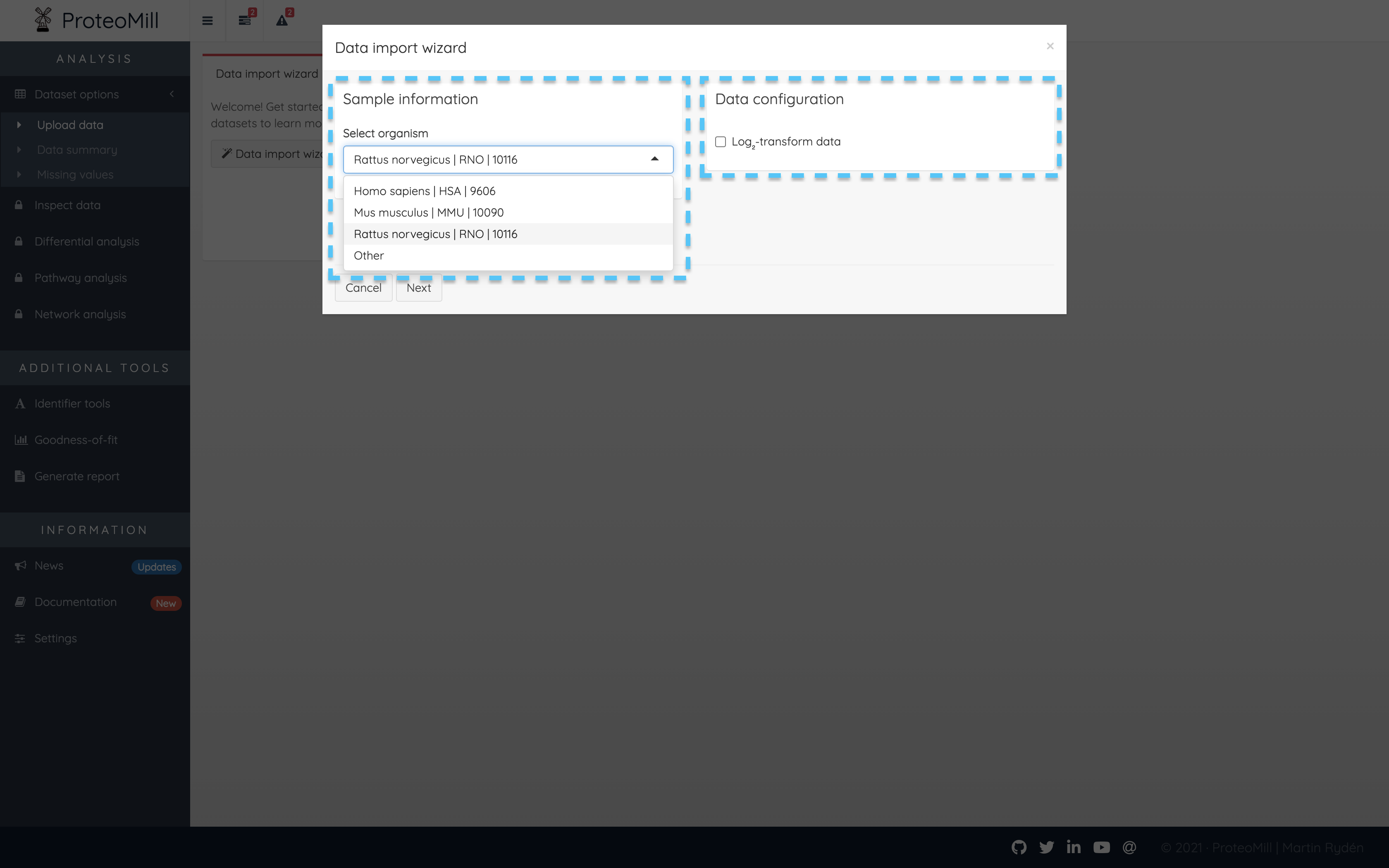
Figure 2.2: Data import wizard
For the next step, your data needs to be in the correct format. ProteoMill accepts expression matrices of protein/gene counts/intensities obtained from LC-MS, RNA-seq or microarray. The file extension should be csv, tsv or txt. Here is a checklist to ensure your file has the correct format.
- Experiment must contain at least two groups/treatments
- Each treatment must contain at least two replicates
- File must have a header row
- First column should contain protein IDs
- Column two and onwards should contain sample names
- Sample names should be in the form treatment_replicate
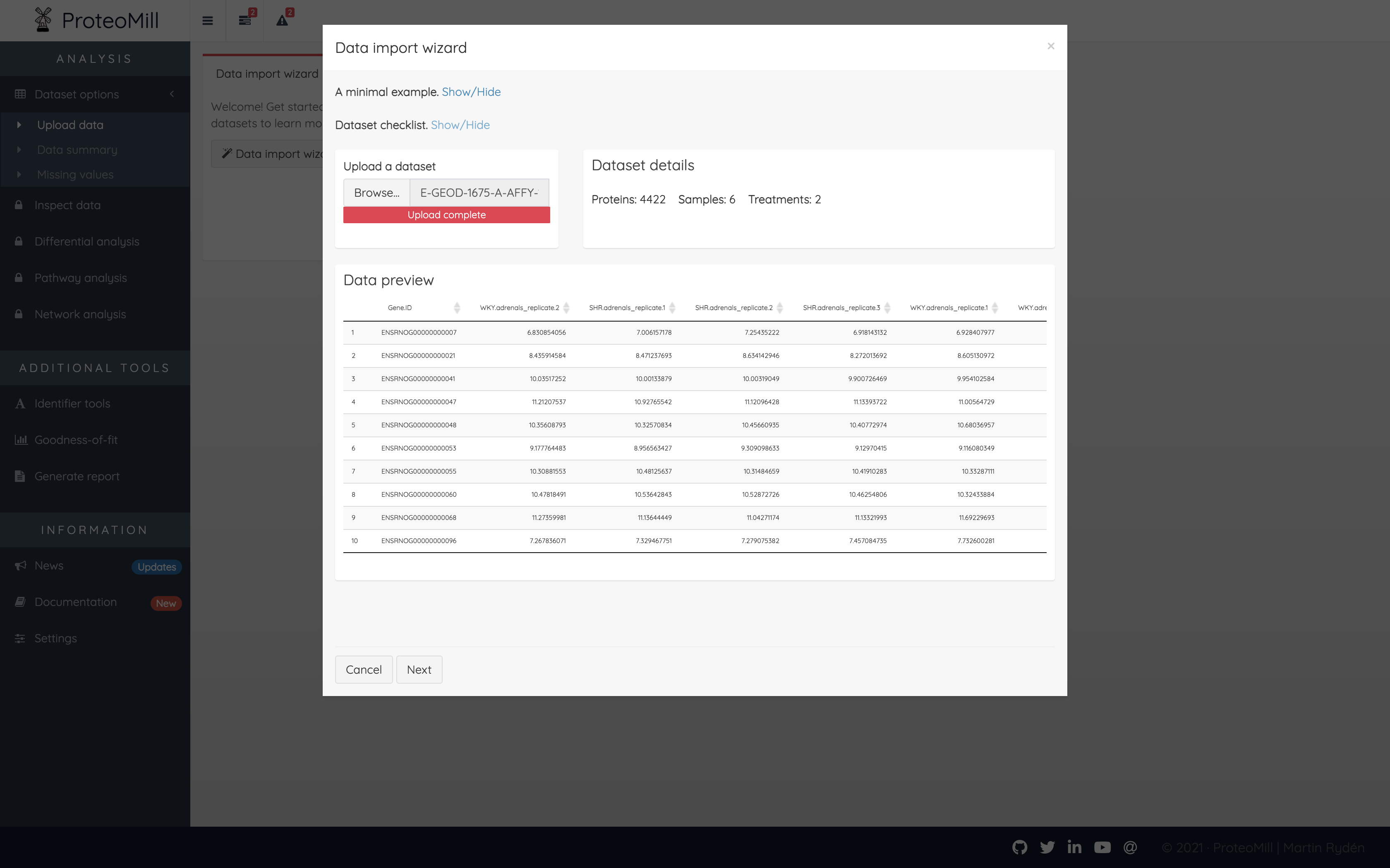
Figure 2.3: Upload dataset
Click Next again to finalize data upload.
2.1.2 Data summary
This section shows an overview of your data. The number of proteins, samples and treatments in your dataset. You may want to revisit this the Data summary page after filtering out proteins with many missing values.
Mapped IDs shows you how many identifiers (protein “labels”) we could recognize. Usually, only the identifier type used in the dataset will be 100%. In the example below, a dataset with 4422 proteins used Ensembl gene ID as identifier type. ProteoMill recognized all 4422 ids, but could only map ~90% of identifiers to other types. This is usually because there is not a 1:1 mapping between identifier types. It could also be the result of identifiers being obsolete (outdated / modified). For UniProt identifiers, ProteoMill offers a tool to check if the identifiers in your dataset are obsolete (please note that this tool is very slow, because it scrapes information from uniprot.org). You find this tool under Identifier tools.
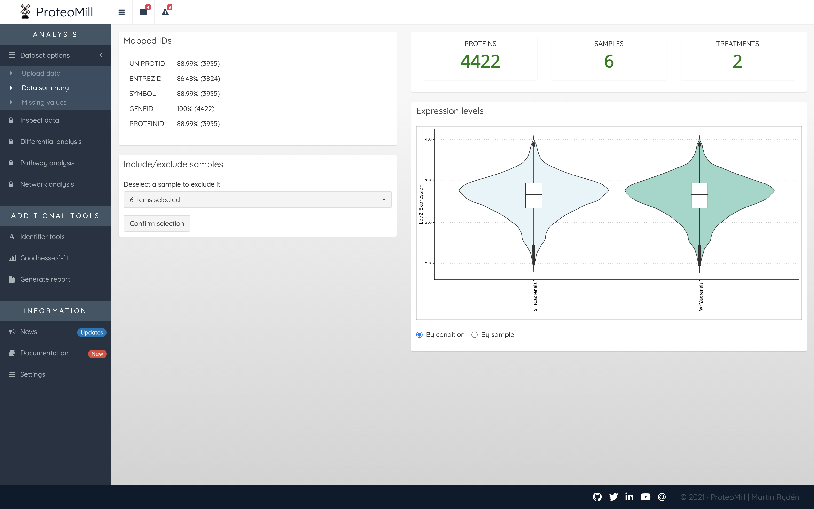
Figure 2.4: Data summary
The Data summary page also lets you exclude samples (perhaps you have discovered a faulty sample in the Data inspection). In the menu, click on a sample to deselect it. Then click on Confirm selection. Note that this does not modify the input file in any way. In order to restore the sample however, you will need to upload your dataset again.
The violin plots presented in the Expression levels box show the (logarithmized) expression levels of each treatment or sample (depending on selection). Violin plots combine box plots and kernal density plots and describes the distribution patterns of your dataset.
2.1.3 Missing values
Missing values are abundant in datasets derived from LC-MS (particularly DDA) and often occur when a peptide’s intensity is below the detection limit. You may want to exclude proteins that have too many missing values to be informative in the differential expression analysis. As a rule of thumb, it is a good idea to exclude the protein if abundances are missing from >= 10% of samples. In ProteoMill, you can select the maximum number of missing values per treatment as a cutoff for each protein.
For example, suppose we have a dataset with ten proteins and two treatments with three replicates each. The dataset has some missing values (NA).
##                a_1       a_2       a_3       b_1       b_2       b_3
## ProteinA        NA 11.419961 10.388858 10.215915  9.040858  9.722175
## ProteinB 11.388863 10.969761  8.496261 10.385133 10.664470        NA
## ProteinC 10.649010 11.904256 10.838549  9.630510 10.507817  9.281374
## ProteinD 11.477876        NA  9.167286        NA  9.313609  9.931160
## ProteinE 10.438720 11.778028 10.785191        NA        NA  9.561443
## ProteinF 10.522318 10.206227 11.800682 10.247542  9.941459  9.427944
## ProteinG  9.955392  8.453688        NA 10.745600 10.438678  9.657005
## ProteinH        NA 10.646198  8.649589 10.341993  9.119790 10.964108
## ProteinI        NA 11.557704  9.655393  9.226342 10.926674 10.595659
## ProteinJ 10.225640  8.039057  9.731437  9.504348 10.014774  9.410400
Let’s inspect the missing values plot.
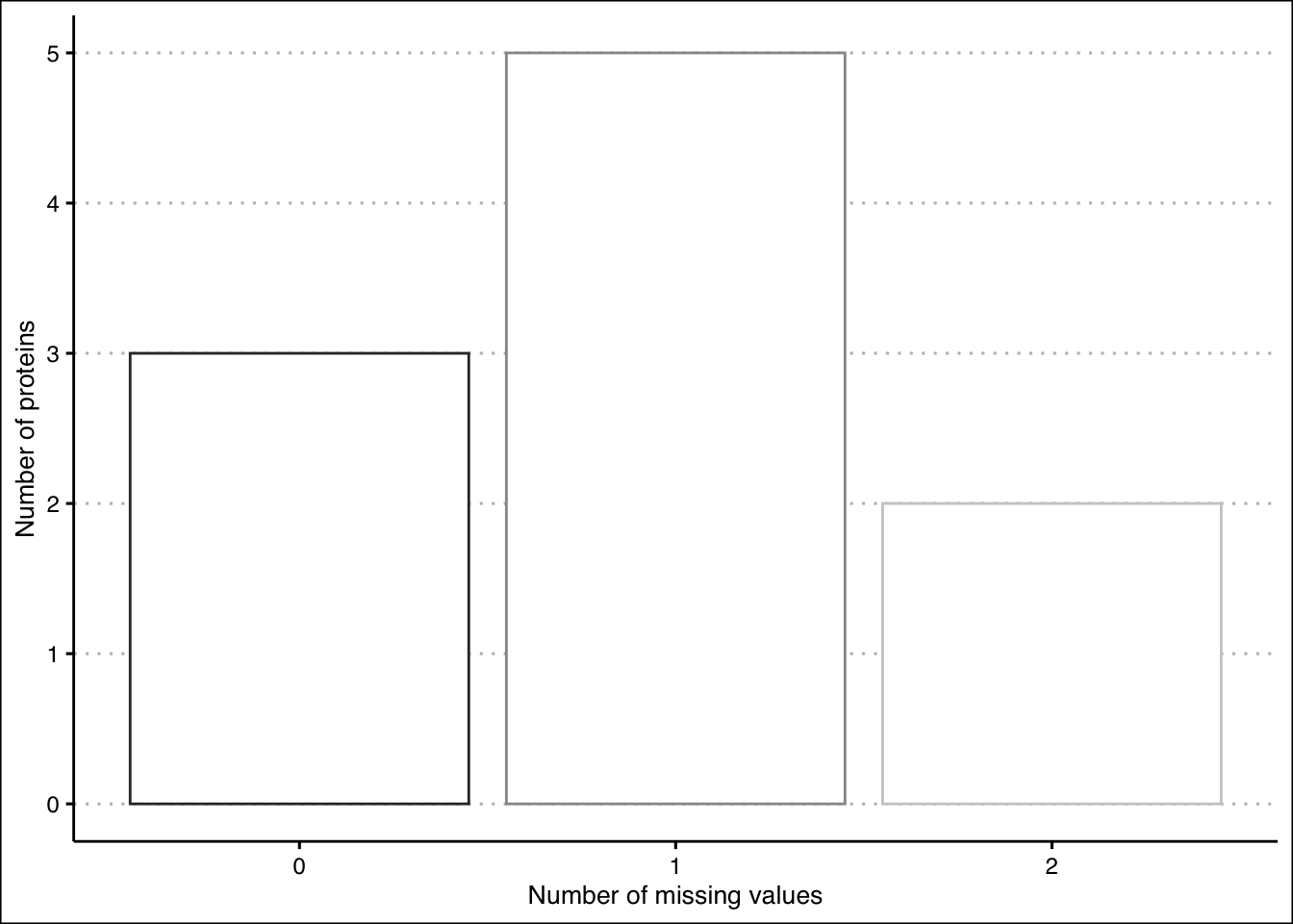
Figure 2.5: Missing values plot before setting a cutoff
The majority of proteins have one missing value. In the dataset we can see that ProteinD and ProteinE both have two missing values. We will set our cutoff to allow for one missing value per treatment. This means we will keep ProteinD because it has only one missing value in a and one missing value in b. ProteinE, however, will be removed, because it has two missing values in b, and we decide that it can no longer be considered informative.
##                a_1       a_2       a_3       b_1       b_2       b_3
## ProteinA        NA 11.419961 10.388858 10.215915  9.040858  9.722175
## ProteinB 11.388863 10.969761  8.496261 10.385133 10.664470        NA
## ProteinC 10.649010 11.904256 10.838549  9.630510 10.507817  9.281374
## ProteinD 11.477876        NA  9.167286        NA  9.313609  9.931160
## ProteinF 10.522318 10.206227 11.800682 10.247542  9.941459  9.427944
## ProteinG  9.955392  8.453688        NA 10.745600 10.438678  9.657005
## ProteinH        NA 10.646198  8.649589 10.341993  9.119790 10.964108
## ProteinI        NA 11.557704  9.655393  9.226342 10.926674 10.595659
## ProteinJ 10.225640  8.039057  9.731437  9.504348 10.014774  9.410400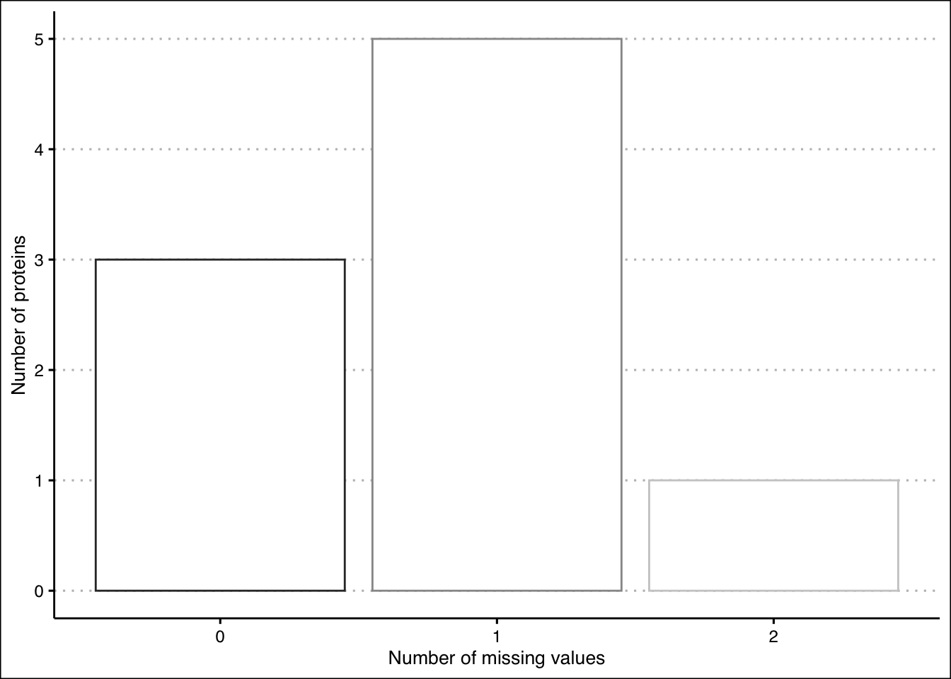
Figure 2.6: Missing values plot after setting a cutoff
If you want to proceed without removing any proteins (despite them having missing values), set the cutoff to a number higher than the number of samples / treatments.
Finishing this step will unlock two new menus and let us continue our analysis.
References
Lazar C, Gatto L, Ferro M, Bruley C, Burger T. Accounting for the Multiple Natures of Missing Values in Label-Free Quantitative Proteomics Data Sets to Compare Imputation Strategies. J Proteome Res. 2016;15:1116–25.
Wang J, Li L, Chen T, Ma J, Zhu Y, Zhuang J, et al. In-depth method assessments of differentially expressed protein detection for shotgun proteomics data with missing values. Sci Rep-uk. 2017;7:3367.
2.2 Inspect data
2.2.1 PCA
Prinipal component analysis (PCA) is an important tool for reducing complexity of multidimensional datasets. Let’s take a look at a dataset that has two treatments and six replicates.
First we’ll inspect the scree plot. This plot tells us the number of components that are of relevance to our PCA. Each principal component in the screen plot is less informative than the previous one in terms of how much variation is explained. What we are typically looking for is a steep drop to be able to determine where which principal components are of value to our analysis. In the example below, this is not perfectly clear.
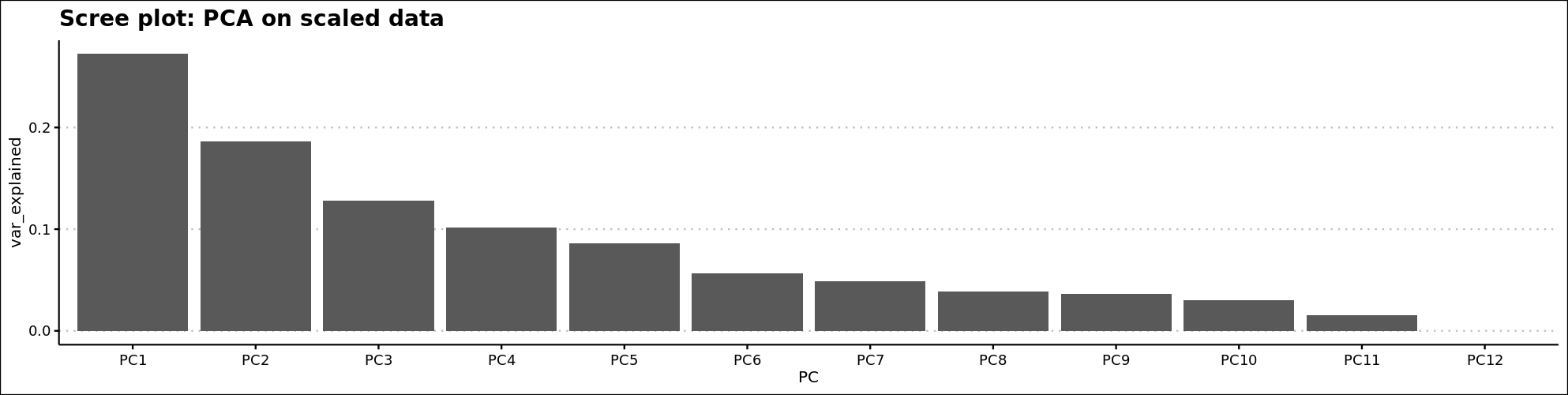
Figure 2.7: Scree plot
Next, we’ll inspect the main PCA window. PCA clusters the samples based on their similarity. This plot shows the two most informative components on the X- and Y-axis.
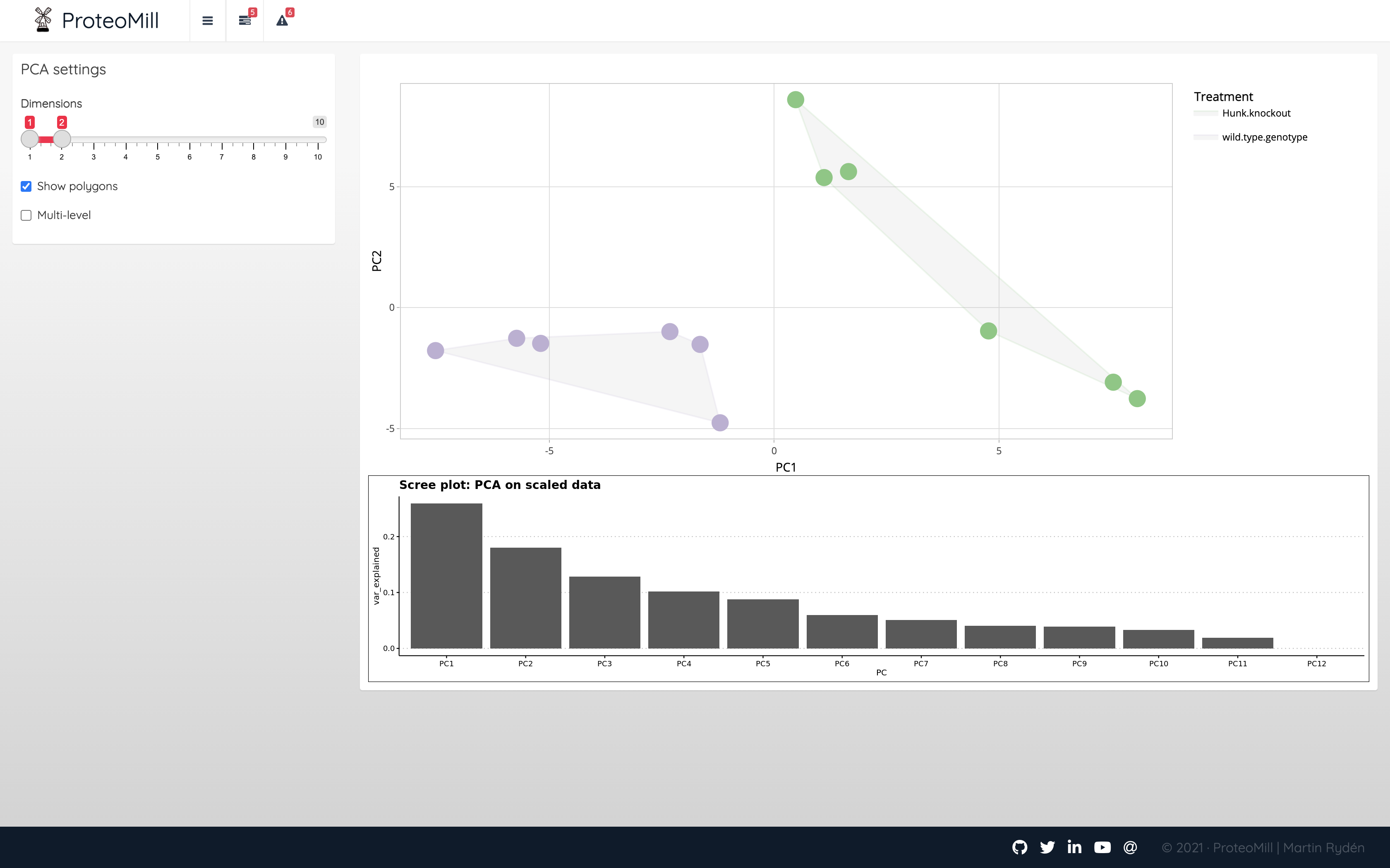
Figure 2.8: PCA 2D
In ProteoMill it is possible to view PCA as a three-dimensional plot. Use the scree plot to determine whether this is useful.
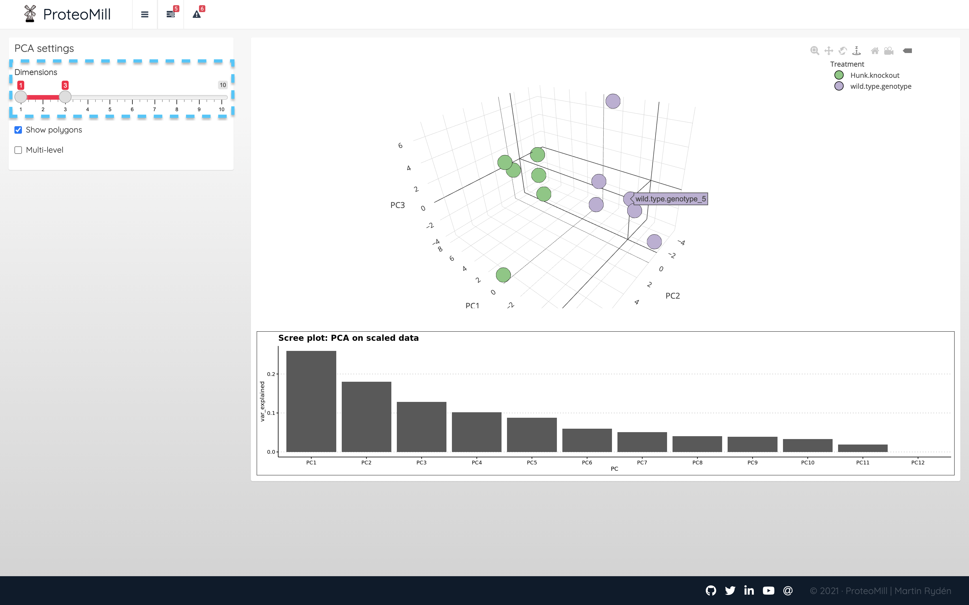
Figure 2.9: PCA 3D
In the above example, there was no clear “steep hill” from which we can decide a cutoff. We can however inspect additional components by dragging the Dimensions slider.
2.2.2 Sample correlation heatmap
Sample-sample correlation heatmap is a useful tool for identifing patterns of similarity or dissimilarity across samples, as well as detecting outliers.
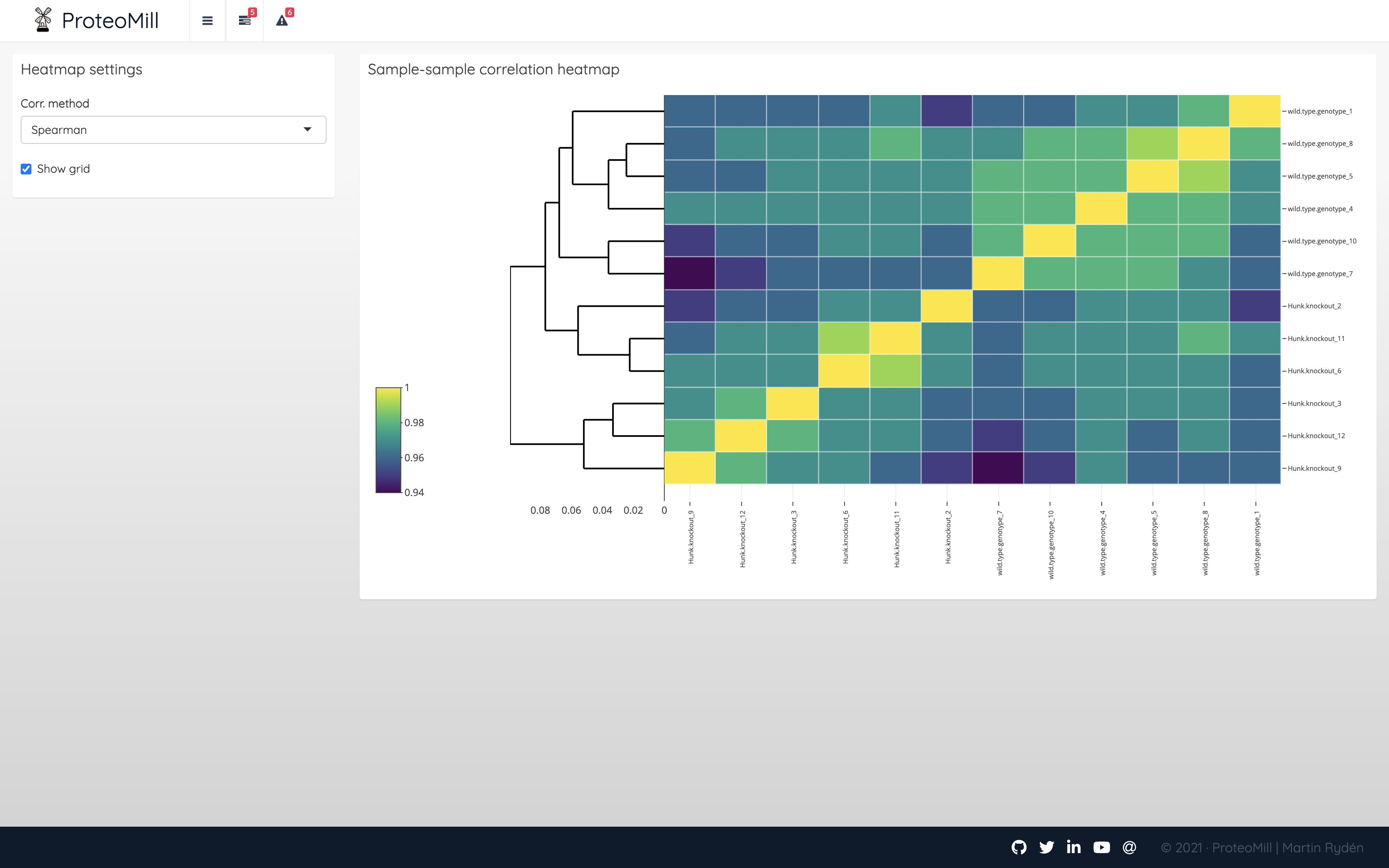
Figure 2.10: Sample correlation heatmap
2.3 Differential expression analysis
A word of caution: do not blindly trust the results generated in ProteoMill as a biological truth. There are many variables that affect the outcome of a biological experiment and such an outcome cannot never be appropriately described by a p-value. Please keep this in mind when you evaluate the results. ProteoMill was designed as an exploratory analysis tool as a method for life science researchers to gain quick insights about their data.
2.3.1 Set a contrast
Differential expression analysis is the process we use to test if there are quantitative changes in expression levels between two treatments. Set the contrasts and specify if the statistical test should adjust for paired samples. There are two packages available for differential expression: DESeq2 which often is the appropriate choice for RNA-seq experiments, and limma, which is a good choice for microarray and LC-MS data.
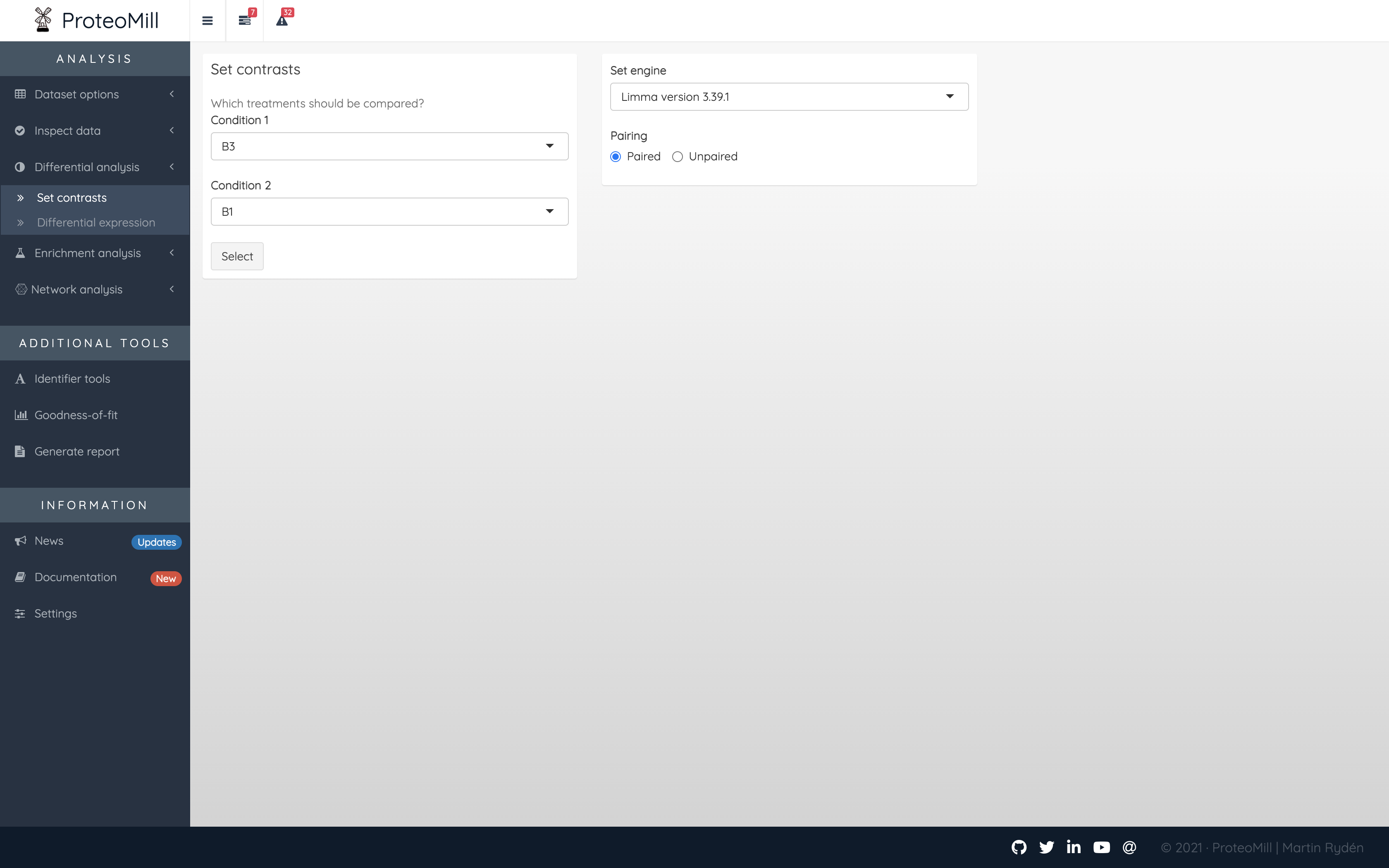
Figure 2.11: Differential expression contrasts
2.3.2 Differential expression results
The results are presented both as a table and as a volcano plot. The results in the table can be filtred by fold-change and by adjusted P-values (FDR). A positive log2 fold change for a protein means the protein is up-regulated in contrast one. A negative log2 fold-change means the protein is down-regulated in contrast one.
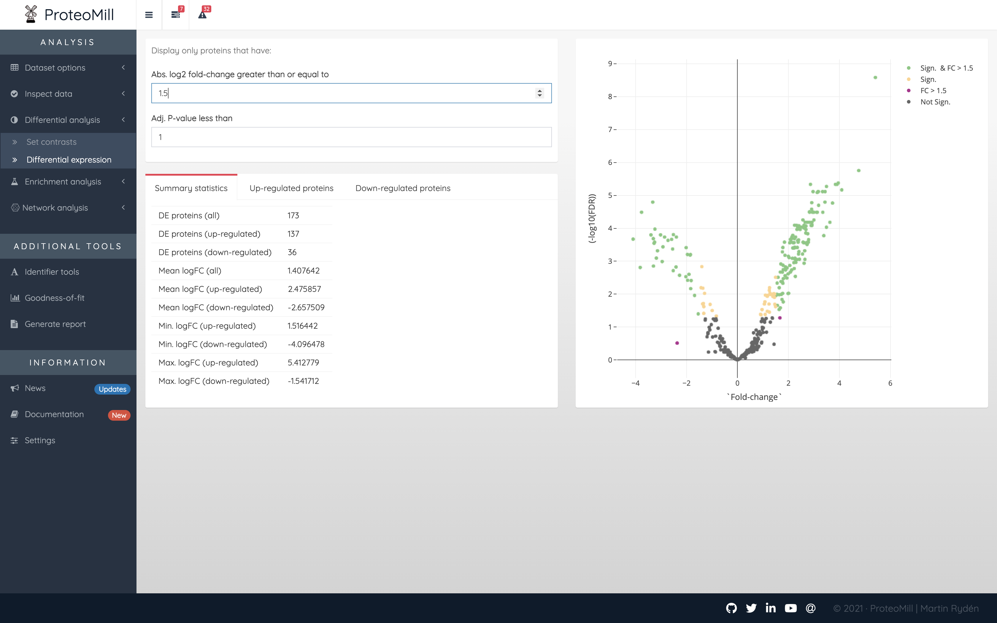
Figure 2.12: Differential expression results
Every point in the volcano plot represents a protein. Its position on the X-axis is a measure of effect size – the greater the value (in positive or negative direction, the more up- or down-regulated, respectively, the protein is in the set contrast), and on the Y-axis a measure of uncertainty – the higher the number the more confident we are in the result.
The volcano plot is color annotated into one to four groups:
- Not Sign. the protein has a FDR >= 0.05 and a log2 fold-change <= 1.5
- FC > 1.5 the protein has a FDR >= 0.05 but a log2 fold-change > 1.5
- Sign. the protein has a FDR < 0.05 but a log2 fold-change <= 1.5
- Sign. and FC > 1.5 the protein has a FDR < 0.05 and a log2 fold-change > 1.5
In short, the proteins in the Sign. and FC > 1.5 group should be of particular interest for us as it has a high effect size and is significantly differentially expressed.
2.4 Pathway analysis
2.4.1 Pathway enrichment
In this section we take a subset of our data – proteins that show up- or down-regulation in the contrast we set earlier. This subset (let’s refer to it as S from here on) will be our proteins of interest, and we will test if they are overrepresented in any protein sets we refer to as pathways. In other words, the question we pose is: which pathways, if any, have a greater number of S-proteins than “expected”?
First, let’s look at the main results table and explain each column.
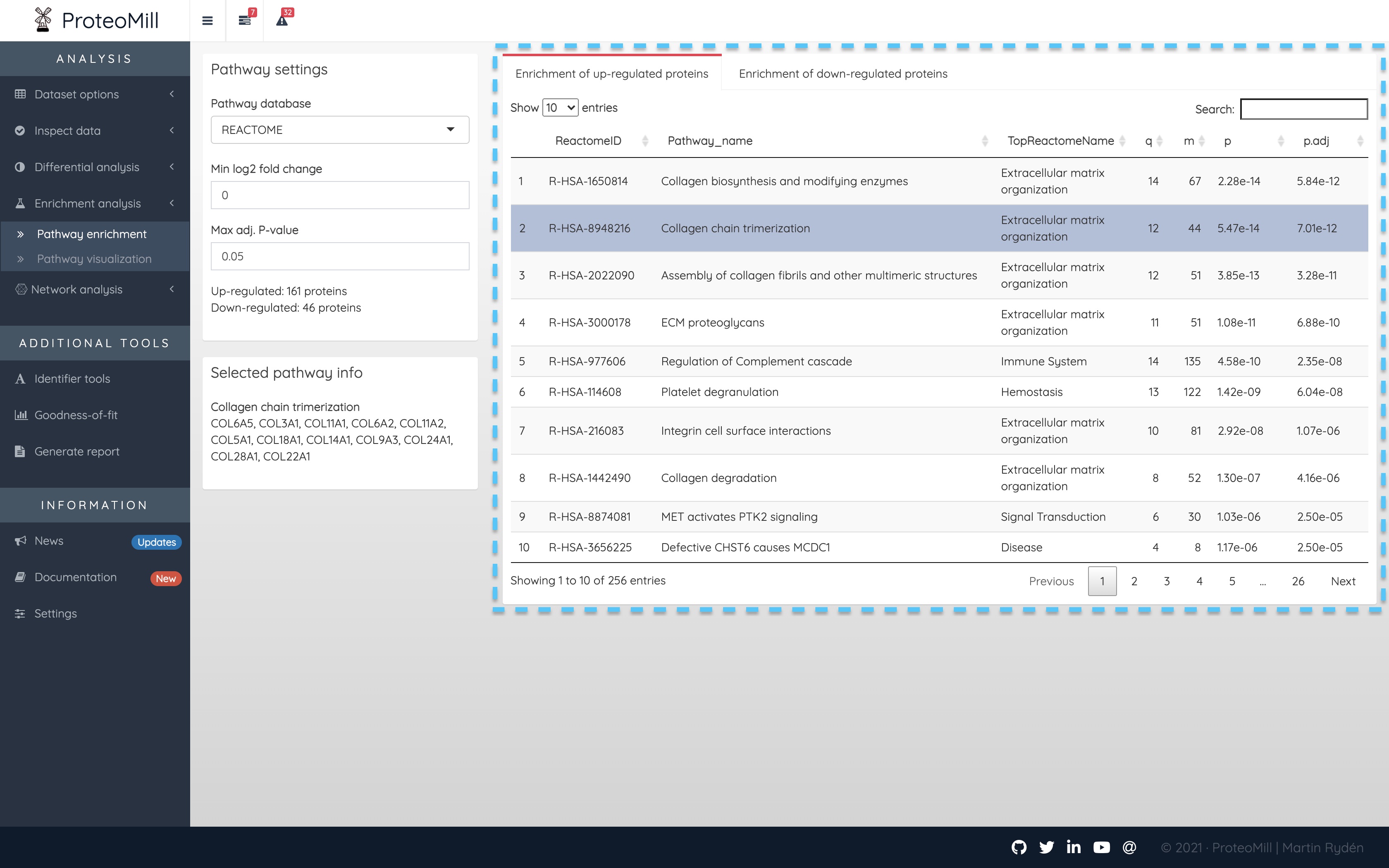
Figure 2.13: Pathway analysis
- ReactomeID - The pathway annotation database used here is called Reactome. ReactomeID is the unique identifier for a given pathway.
- Pathway_name - This column displays the name of the pathway for which we have tested overrepresentation of our protein set.
- TopReactomeName - Reactome organizes their pathways in a hierarchical structure. This column is the top-level parent of Pathway_name in that hierarchy. We include it here as a general biological categorization of the pathway.
- q - This is the number of proteins from S that overlap with proteins annotated to the pathway.
- m - This is the total number of proteins annotated to the pathway.
- p - The p-value is our evidence agains the null hypothesis for this test: there is no association between a pathway’s annotated proteins and the studied contrast.
- p.adj - We have to correct for the fact that we repeat this test for each protein, so p.adj is how we decide which pathways are enriched (show association to the studied phenotype).
Clicking on a pathway will show the proteins from S that overlap with proteins annotated to the pathway (i.e. how we calculate q). This list of proteins will appear under Selected pathway info.
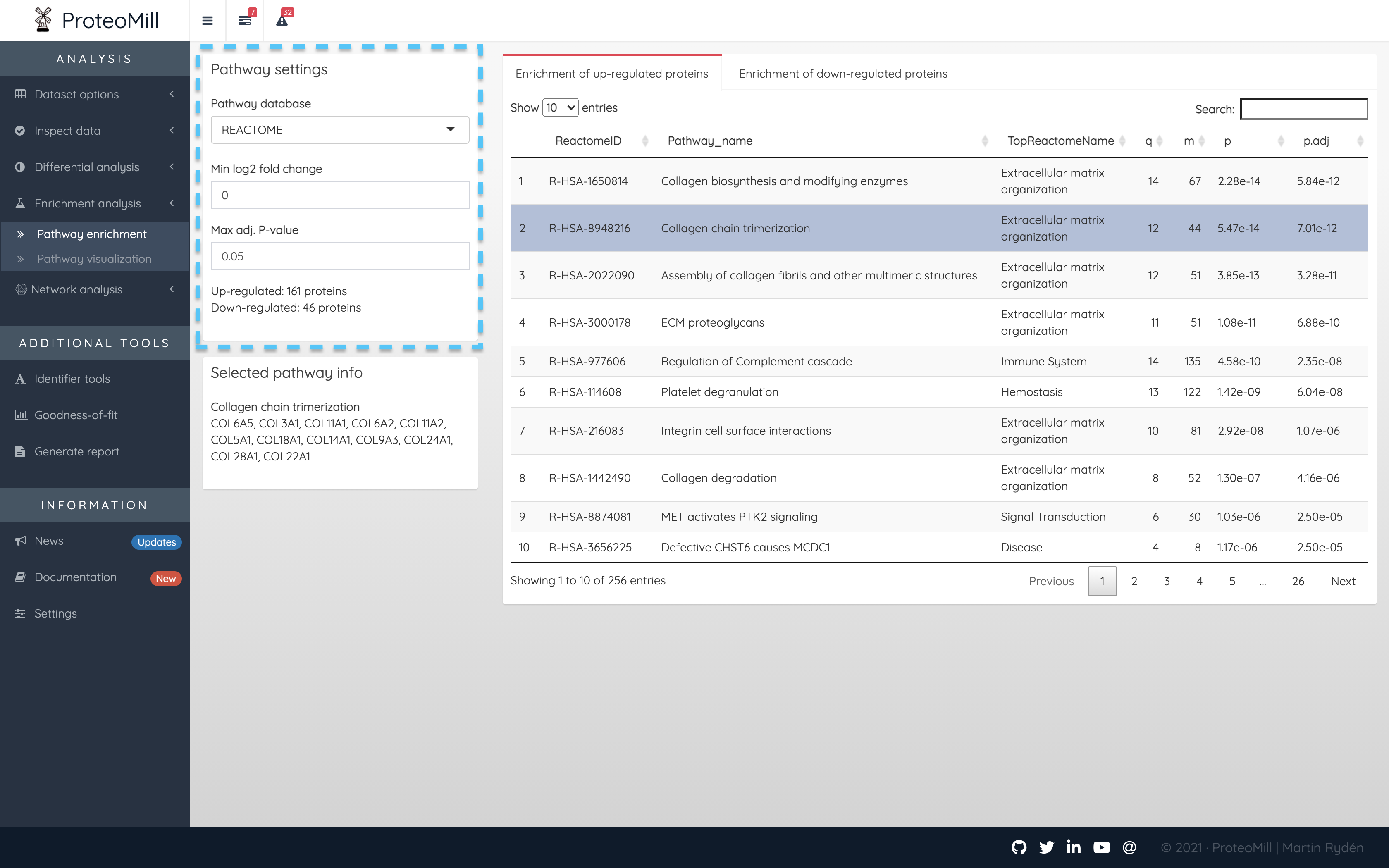
Figure 2.14: Pathway analysis
In the Pathway settings box you can control which proteins from the differential expression results should be included in the pathway analysis. The conventional approach is to take a subset based on a p-value threshold. In ProteoMill you may choose to subset by (absolute, log2) fold-change and/or (adjusted) p-value. In the example above, we have set a p-value threshold at 0.05, i.e. proteins with an adjusted p-value of < 0.05 will be our S. In this scenario, fold-change will be ignored. If the “Min log2 fold change” was set to 1, there would be the additional requirement that proteins must have a log2 fold-change of more than 1 OR less than -1.
2.4.2 Pathway visualization
If there are no significantly over-represented pathways, this is where the analysis ends.
Otherwise, we will revisit the volcano plot that we say in the differential expression analysis, now annotated with pathways. If a protein is significantly over-represented in a pathway, it will be color annotated with that pathway. This plot that now contains information collected from both differential expression analysis and pathway analysis will be useful in the next step major section, where we conduct protein-protein interaction analysis.
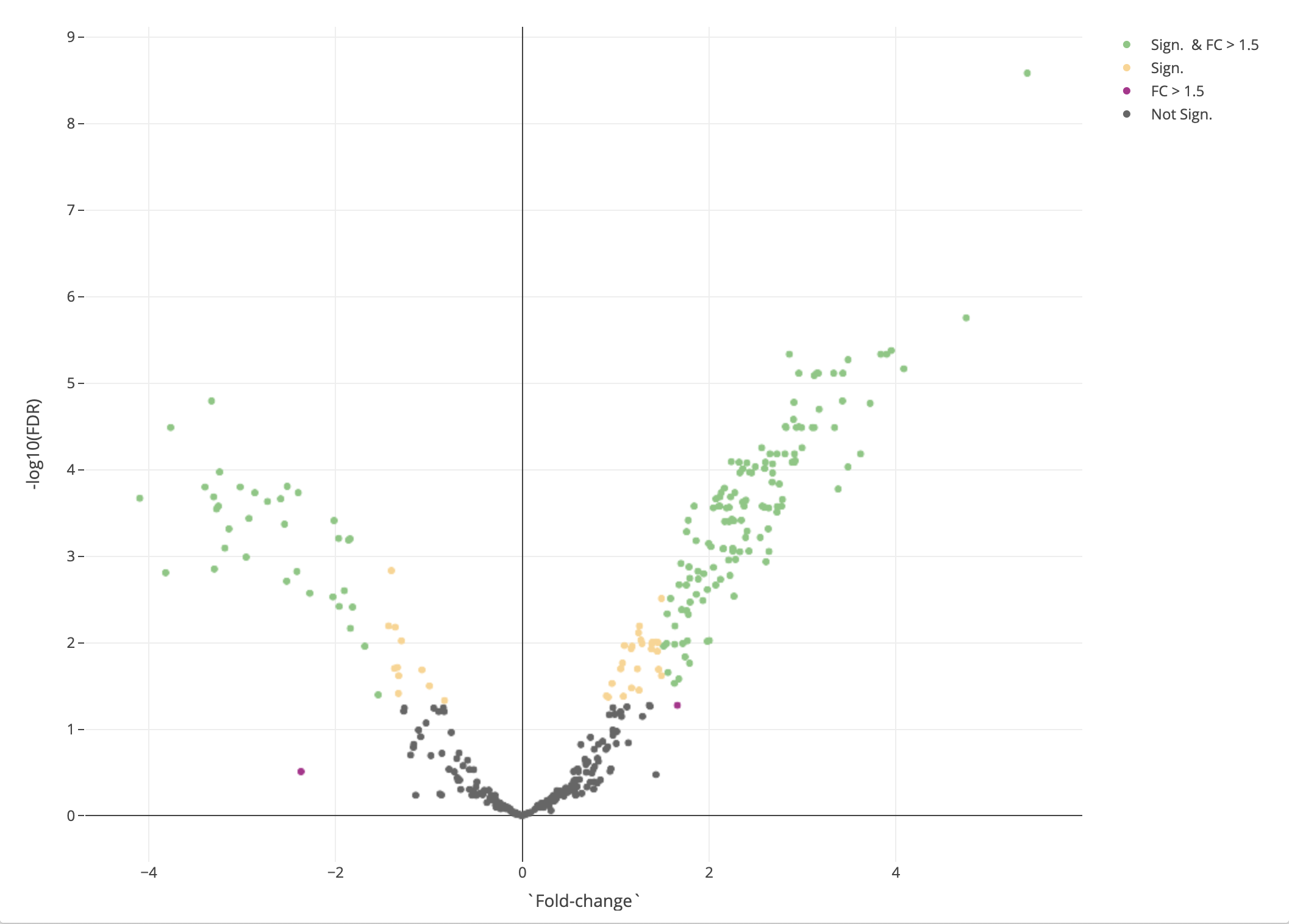
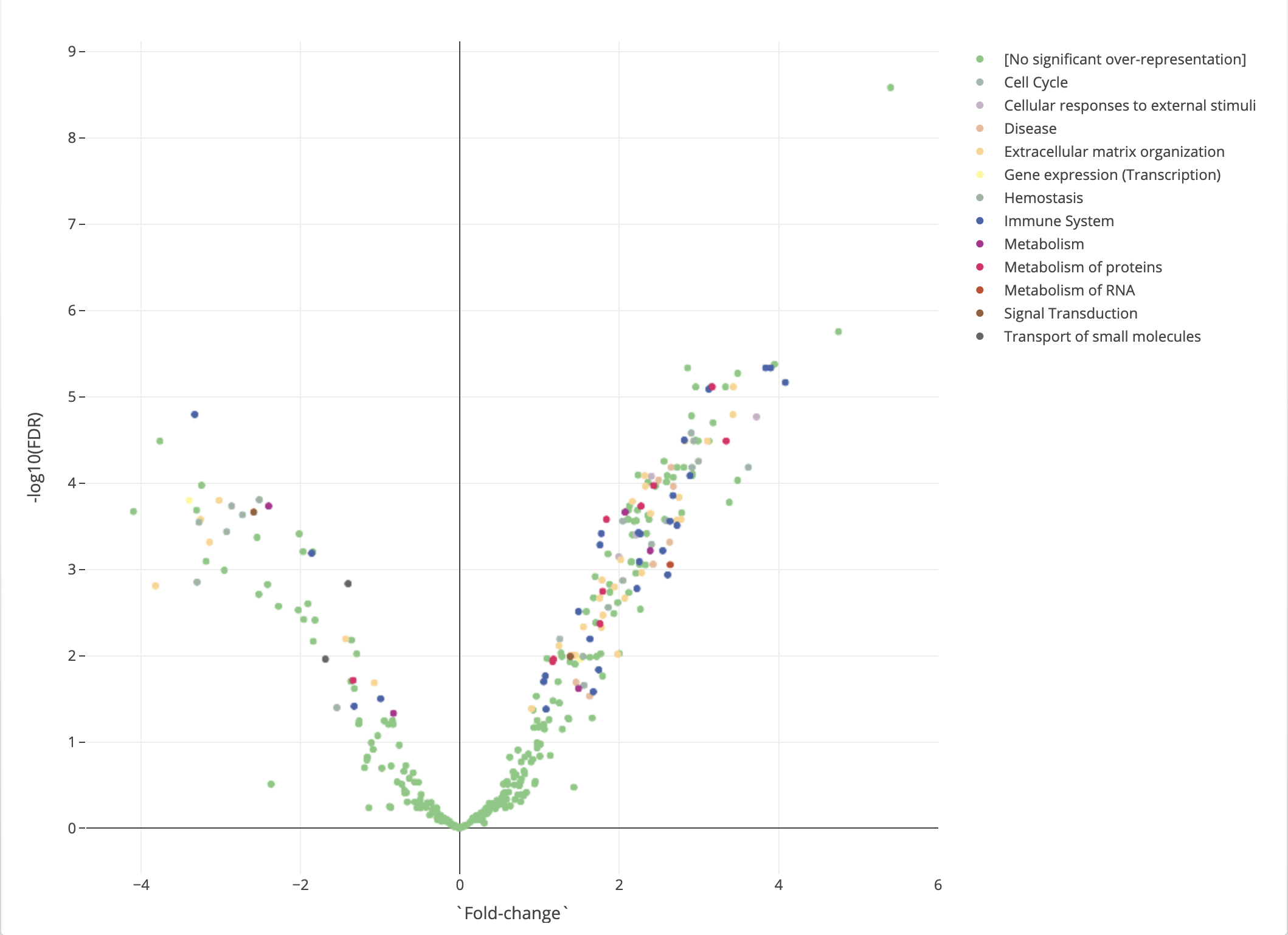
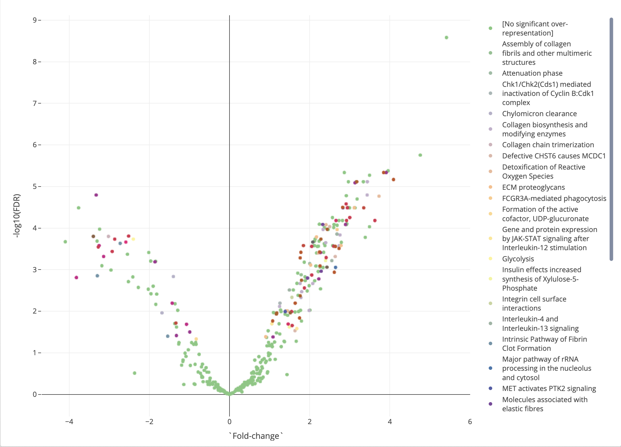
Figure 2.15: Pathway analysis
2.5 Network analysis
In this final part of the analysis pipeline, we make use of all the information about the proteins we have collected up until this point. On our right is the volcano plot, where each point represents a protein. Its position on the X-axis is a measure of effect size – the greater the value (in positive or negative direction, the more up- or down-regulated, respectively, the protein is), and on the Y-axis a measure of uncertainty – the higher the number the more confident we are in the result.
There are three annotation modes for the proteins: by differential expression groups, by enrichment results (top-level pathway), or enrichment results (pathway). These colors will be mirrored in the network plot (left).
Every protein in the Volcano plot, corresponds to a protein in the network plot. The plots are interconnected, meaning we can use the volcano plot for extracting subnetworks of interest. This is useful because the volcano plot now contains a great deal of information about the proteins. Is it highly up- or down-regulated? Can we place it in a molecular context, i.e. describe it as over-represented in a pathway? Are there other “members” of said pathway that we expect it to interact with? The volcano plot can suggest answers to these questions.
In the Network plot, we keep the color annotation, but replace the information on fold-change and FDR with another dimension: the interaction of proteins, represented by the links, or edges, between the protein nodes. A protein and its links will be visible in the network plot only if it fulfills the requirements specified in the Network settings box. In the example below, we have defined a low threshold for (absolute, log2) fold-change from there differential expression results, in order to exclude proteins that showed close to no up- or down-regulation.
We have set the Interaction confidence to 7/10 which means we have moderately good amounts of evidence in support of the interactions being presented. For non-human species, the availability of interaction data is much poorer, and we therefore suggest using a lower interaction confidence value.
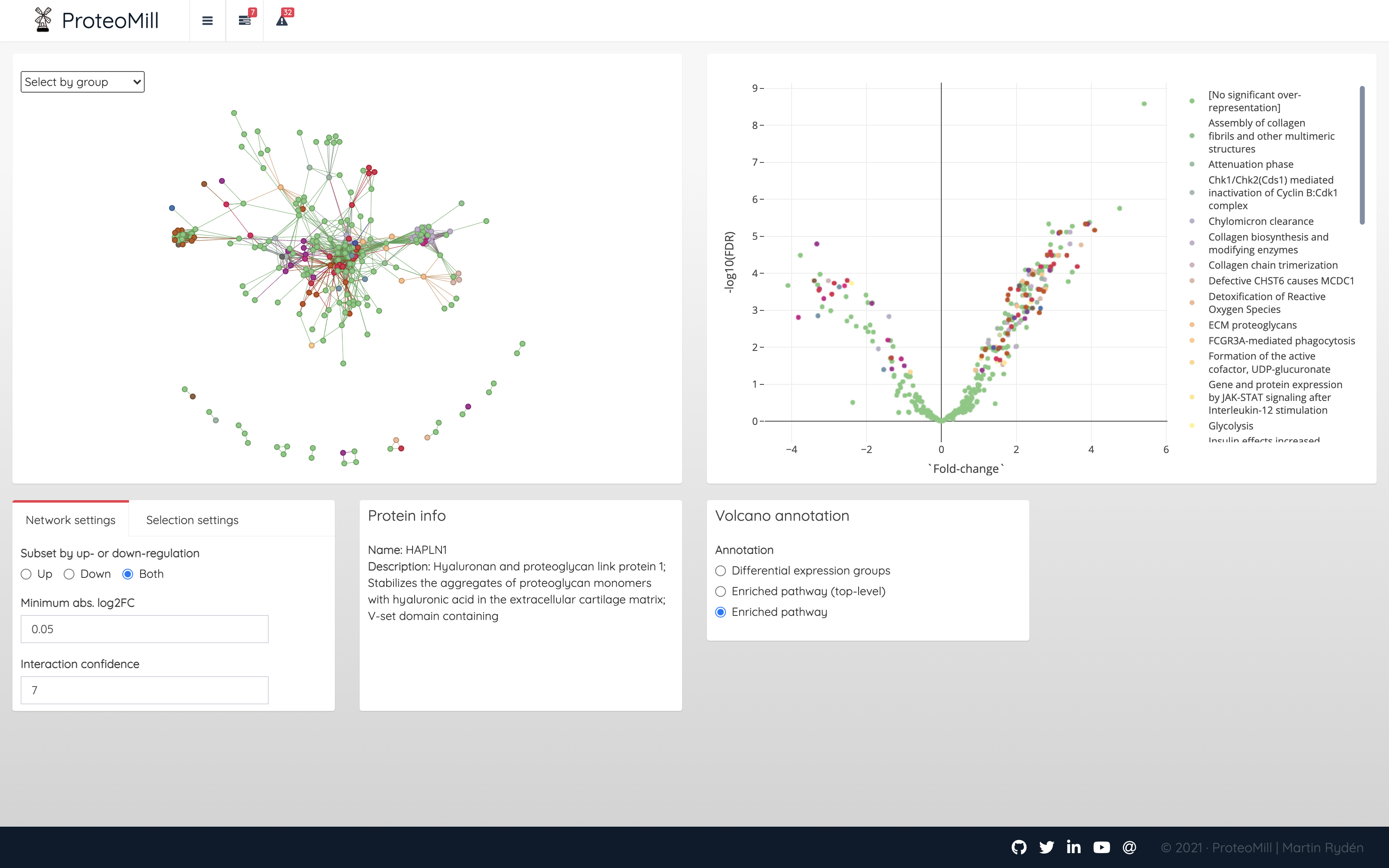
Figure 2.16: Network analysis overview
A unique feature in ProteoMill is that you can make a selection in the volcano plot (using the Plotly tools Box Select or Lasso Select). If Selection mode is set to “Strict”, the network will only show the interaction of proteins within the selection.
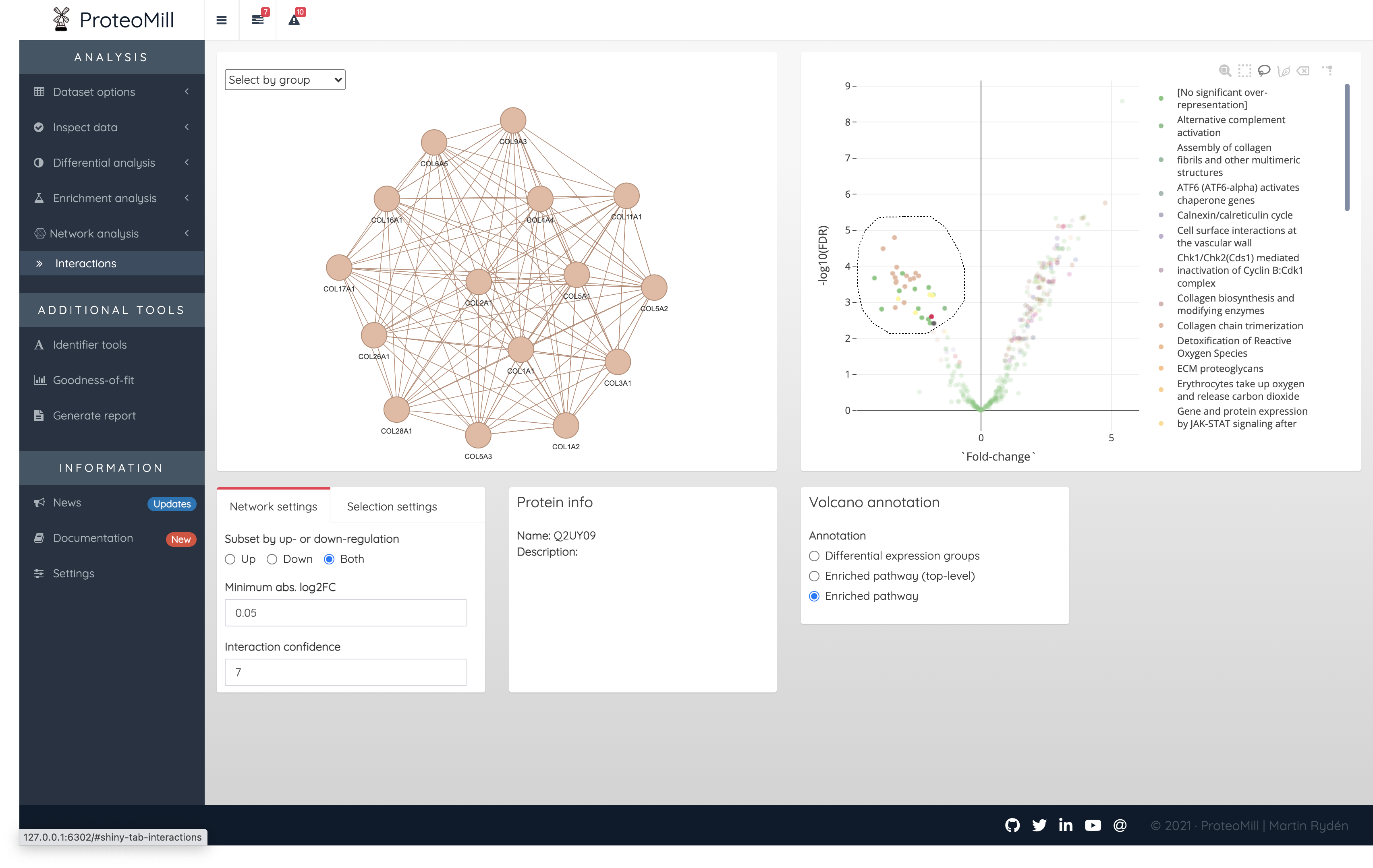
Figure 2.17: Network analysis. Using Selection mode ‘Strict’, the only interactions within the selection formed a collagen cluster subnetwork.
If instead the Selection mode is set to “Extended”, the network will show the all interactions between the selection and any other protein in the uploaded dataset.
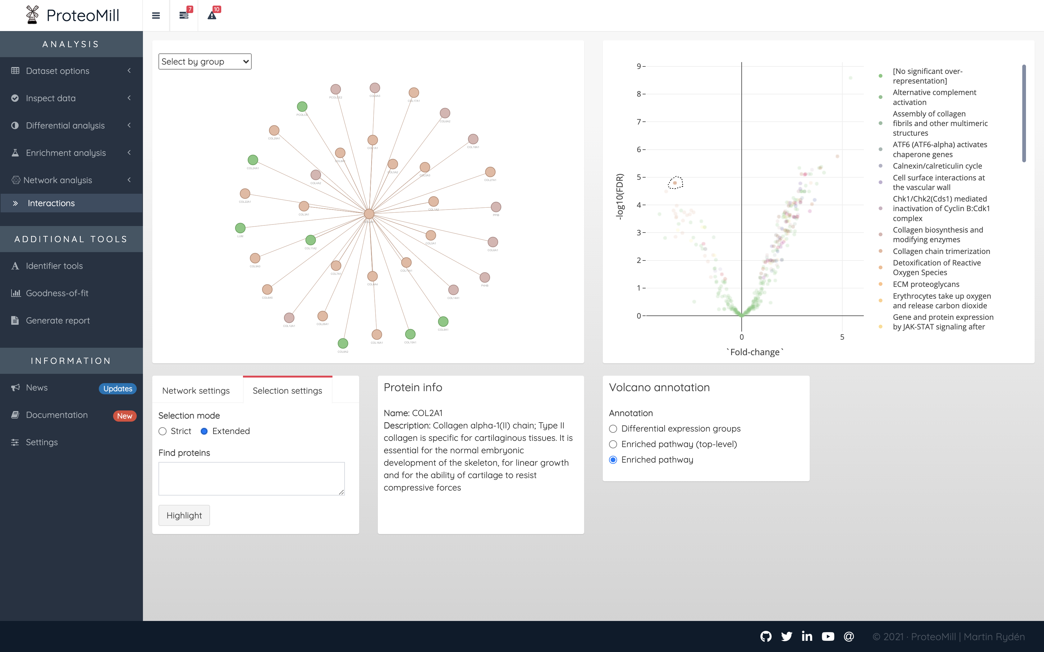
Figure 2.18: Network analysis. Using Selection mode ‘Extended’, we can see all proteins (from the uploaded dataset) that have interactions with our selection.