Note 3 Simulation Example on Structural Equation Modeling (SEM)

# Load required packages
library(tidyverse)
theme_set(theme_classic() +
            theme(panel.grid.major.y = element_line(color = "grey92")))

3.1 Simulate Multivariate Data

In SEM, when multivariate normality is assumed, one can either generate data directly using matrix algebra, or generate the latent variables first before generating the observed variables. The first method is faster, but the second method is more general and can be applied to situations like categorical data or multilevel data. Therefore, in this note we’ll use the second method.

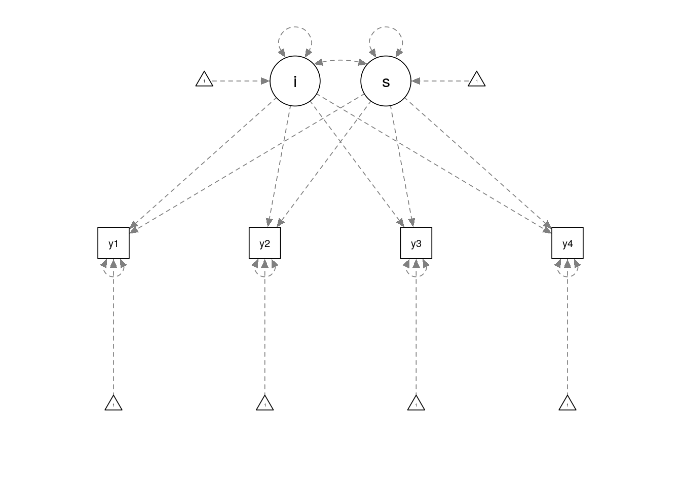
Let’s do a latent growth model (LGM) similar to the one in the note “Simulating Multilevel Data.” Here is the model in a latent growth model representation: \[\begin{bmatrix} y_{0i} \\ y_{1i} \\ y_{2i} \\ y_{3i} \end{bmatrix} = \boldsymbol{\mathbf{\Lambda }} \begin{bmatrix} \eta_{1i} \\ \eta_{2i} \end{bmatrix} + \begin{bmatrix} e_{0i} \\ e_{1i} \\ e_{2i} \\ e_{3i} \end{bmatrix}\] where \(y_{0i}, \ldots, y_{3i}\) are the outcome values for person \(i\) from time 0 to time 3, \(\eta_{1i}\) is the specific intercept for person \(i\), \(\eta_{2i}\) is the specific slope for person \(i\), and \(e_{0i}, \ldots, e_{3i}\) are the within-person level error term. The distributional assumptions are

\[\begin{align*} \begin{bmatrix} \eta_{1i} \\ \eta_{2i} \end{bmatrix} & \sim \mathcal{N}\left(\begin{bmatrix} \alpha_1 \\ \alpha_2 \end{bmatrix}, \begin{bmatrix} \phi_{11} & \phi_{21} \\ \phi_{21} & \phi_{22} \end{bmatrix}\right) \\ \begin{bmatrix} e_{0i} \\ e_{1i} \\ e_{2i} \\ e_{3i} \end{bmatrix} & \sim \mathcal{N}\left(\begin{bmatrix} 0 \\ 0 \\ 0 \\ 0 \end{bmatrix}, \begin{bmatrix} \theta_{11} & 0 & 0 & 0 \\ 0 & \theta_{22} & 0 & 0 \\ 0 & 0 & \theta_{33} & 0 \\ 0 & 0 & 0 & \theta_{44} \\ \end{bmatrix}\right) \end{align*}\]

A path diagram is shown below:

growth_model <- "i =~ 1*y1 + 1*y2 + 1*y3 + 1*y4
                 s =~ 0*y1 + 1*y2 + 2*y3 + 3*y4
                 i ~~ 1 * i
                 s ~~ 0.2 * s + 0.1 * i
                 y1 ~~ 0.5 * y1
                 y2 ~~ 0.5 * y2
                 y3 ~~ 0.5 * y3
                 y4 ~~ 0.5 * y4
                 i ~ 1 * 1
                 s ~ 0.5 * 1"
library(semPlot)
semPaths(semPlotModel_lavaanModel(growth_model))

3.1.1 Using R

Here’s the code for generating the data:

library(mnormt)
set.seed(123)
# Define sample size
N <- 100
# Define the Fixed Parameters
alpha <- c(1, 0.5)  # latent means
Phi <- matrix(c(1, 0.1, 
                0.1, 0.2), nrow = 2)  # latent variances/covariances
Lambda <- cbind(c(1, 1, 1, 1), 
                c(0, 1, 2, 3))  # factor loadings
Theta <- diag(0.5, nrow = 4)
# Generate latent factor scores
eta <- rmnorm(N, mean = alpha, varcov = Phi)
# Generate residuals:
e <- rmnorm(N, varcov = Theta)
# Compute outcome scores: y_i = t(Lambda %*% eta_i) + e
y <- tcrossprod(eta, Lambda) + e
# Make it a data frame
colnames(y) <- paste0("y", 1:4)
df <- as.data.frame(y)

If you want to check whether the simulated data is correct, generate with a large sample size, and check the means and covariances:

N_test <- 1e5
eta_test <- rmnorm(N_test, mean = alpha, varcov = Phi)
colMeans(eta_test)

># [1] 1.0016925 0.5021968

cov(eta_test)

>#          [,1]      [,2]
># [1,] 1.001489 0.1000130
># [2,] 0.100013 0.2011578

e_test <- rmnorm(N_test, varcov = Theta)
colMeans(e_test)

># [1]  0.0008598494  0.0025900286 -0.0051191571  0.0011246080

cov(e_test)

>#               [,1]          [,2]          [,3]          [,4]
># [1,]  0.4995076410 -0.0007194104  0.0010100393 -0.0007624743
># [2,] -0.0007194104  0.4993700934 -0.0016984945  0.0024070969
># [3,]  0.0010100393 -0.0016984945  0.4965962722  0.0003983313
># [4,] -0.0007624743  0.0024070969  0.0003983313  0.5027934517

It’s handy to wrap this as a function:

gen_lgm_data <- function(N, alpha, Phi, Lambda, Theta) {
  # Generate latent factor scores
  eta <- rmnorm(N, mean = alpha, varcov = Phi)
  # Generate residuals:
  e <- rmnorm(N, varcov = Theta)
  # Compute outcome scores
  y <- tcrossprod(eta, Lambda) + e
  colnames(y) <- paste0("y", 1:4)
  # Make it a data frame
  as.data.frame(y)
}
# Test it:
set.seed(123)
gen_lgm_data(100, 
             alpha = c(1, 0.5), 
             Phi = matrix(c(1, 0.1, 
                            0.1, 0.2), nrow = 2), 
             Lambda = cbind(c(1, 1, 1, 1), 
                            c(0, 1, 2, 3)), 
             Theta = diag(0.5, nrow = 4)) %>% 
  head() # shows only the first six cases

>#            y1         y2          y3        y4
># 1 1.994318062 1.71116086  0.93927927 1.8544817
># 2 2.265725727 2.90855563  3.37429135 4.1980646
># 3 2.296655600 2.35159235  3.73462339 5.0831256
># 4 2.332408257 1.09066818  0.74843609 2.6298055
># 5 0.001197646 0.03891746 -0.08691963 0.1158814
># 6 1.818221258 3.44031115  4.56735772 5.0621645

Indeed, you get the same data!

3.1.2 Other methods for generating SEM data

Many SEM software or packages have capability in generating data with input of an SEM model. For example, in R, you can call Mplus using the MplusAutomation package and use their MONTECARLO routine. In R, you can generate SEM data using the lavaan package with the simulateData() function, like the following example:

# Using a previously defined SEM model:
lavaan::simulateData(growth_model) %>% 
  head() # shows only the first six cases

>#          y1         y2        y3         y4
># 1 0.7164342  0.5568492 0.4726109 -0.1122304
># 2 1.8000324  1.8018441 1.5462532  2.4277768
># 3 0.6034256  0.6713423 2.2884345  3.1191797
># 4 1.1521190  2.7229104 4.7980347  5.8445554
># 5 0.6229306 -0.1175073 1.7054730  0.5659889
># 6 0.5230306  2.1871287 2.6141488  2.6783935

Personally, however, I prefer directly simulating data in R because

it forces you to specify everything in the model in the way you want. Especially in Mplus there are a lot of hidden default settings that may mess up with your simulation;
it makes the process of generating data more transparent;
it helps you learn the math behind the model;
it is more flexible as you can specify any distributional assumptions or models not supported by the SEM packages.

3.2 Analyzing the Simulated Data

In R, for running SEM models, the most common options are lavaan, OpenMx, and Mplus (via MplusAutomation). When possible, I’ll stick to lavaan to avoid jumping between programs, so let’s analyze the simulated data twice, first with the true model and second with a misspecified model where the random slope term is omitted (i.e., the variance of s is constrained to zero).

library(lavaan)

># This is lavaan 0.6-3

># lavaan is BETA software! Please report any bugs.

# True model
m1 <- 'i =~ 1*y1 + 1*y2 + 1*y3 + 1*y4
       s =~ 0*y1 + 1*y2 + 2*y3 + 3*y4
       i ~~ s'
# Model without random slopes
m2 <- 'i =~ 1*y1 + 1*y2 + 1*y3 + 1*y4
       s =~ 0*y1 + 1*y2 + 2*y3 + 3*y4
       s ~~ 0*i + 0*s'
m1_fit <- growth(m1, data = df)
m2_fit <- growth(m2, data = df)

Here’s some examples of things you can extract (without showing all the results)

fitMeasures(m1_fit)  # return more than 30 fit indices
# Specific fit indices
fitMeasures(m1_fit, c("chisq", "df", "pvalue", "cfi", "rmsea"))
coef(m1_fit)  # parameter estimates
vcov(m1_fit)  # asymptotic covariance matrix of parameters
# Asymptotic standard errors of latent mean of s
sqrt(diag(vcov(m1_fit))["s~1"])
parameterEstimates(m1_fit, standardized = FALSE)  # coefficients, SE, CI
modificationIndices(m1_fit, minimum.value = 3.84)  # modification indices
# Bootstrapped fit index
bootstrapLavaan(m1_fit, R = 1000L, type = "bollen.stine",
                FUN = fitMeasures, fit.measures = c("cfi"))

3.3 Full Example of a Small Scale Simulation

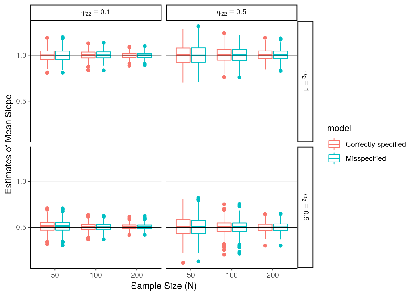
In a methodological experiment with Monte Carlo simulation, one usually generates millions of data sets across tens or hundreds of carefully chosen conditions. As an example, here is a small scale simulation study on LGM. The two goals are: (a) to understand the bias on the mean of slopes and its standard error estimates, and (b) to illustrate the difference between estimated and empirical standard error.

For simplicity, I’ll only choose three designed factors (i.e., manipulated independent variables), namely sample size, variance of the random slope in the data generating model, and the mean of the slopes. The design factors are summarized here:

Sample size (N): 50, 100, 200
Variance of slopes (\(\phi_{22}\)): 0.1, 0.5 (i.e., 1/10 and 1/2 of the intercept variance)
Mean of slopes (\(\alpha_2\)): 1, 0.5

Therefore, it’s a 3 \(\times\) 2 \(\times\) 2 factorial design. Now let’s walk through each component.

3.3.1 Fixed Values for the Study

In the study I decided to run 500 replications for each condition. I can estimate the simulation error to see whether it’s enough.

set.seed(515)  # set the seed for reproducibility
NREP <- 500  # number of replications
# Fixed parameters (all caps)
ALPHA1 <- 1  # latent mean of intercepts
PHI11 <- 1  # intercept variance
LAMBDA <- cbind(c(1, 1, 1, 1), 
                c(0, 1, 2, 3))  # factor loadings
THETA <- diag(0.5, nrow = 4)  # residual variances

We should also define everything that will not change across replications and across conditions, including syntax for running growth models, functions to generate data, etc.

# Function for generating data:
gen_lgm_data <- function(N, alpha, Phi, Lambda, Theta) {
  # Generate latent factor scores
  eta <- rmnorm(N, mean = alpha, varcov = Phi)
  # Generate residuals:
  e <- rmnorm(N, varcov = Theta)
  # Compute outcome scores
  y <- tcrossprod(eta, Lambda) + e
  colnames(y) <- paste0("y", 1:4)
  # Make it a data frame
  as.data.frame(y)
}
# lavaan syntax
# True model
m1 <- 'i =~ 1*y1 + 1*y2 + 1*y3 + 1*y4
       s =~ 0*y1 + 1*y2 + 2*y3 + 3*y4
       i ~~ s'
# Model without random slopes
m2 <- 'i =~ 1*y1 + 1*y2 + 1*y3 + 1*y4
       s =~ 0*y1 + 1*y2 + 2*y3 + 3*y4
       s ~~ 0*i + 0*s'

3.3.2 Keep track of simulation conditions

I’ll create a data frame to store the design factors:

# Design factors:
DESIGNFACTOR <- expand.grid(
  N = c(50, 100, 200), 
  phi22 = c(0.1, 0.5), 
  alpha2 = c(1, 0.5)
)
# Add condition number:
DESIGNFACTOR <- rowid_to_column(DESIGNFACTOR, "cond")
DESIGNFACTOR

>#    cond   N phi22 alpha2
># 1     1  50   0.1    1.0
># 2     2 100   0.1    1.0
># 3     3 200   0.1    1.0
># 4     4  50   0.5    1.0
># 5     5 100   0.5    1.0
># 6     6 200   0.5    1.0
># 7     7  50   0.1    0.5
># 8     8 100   0.1    0.5
># 9     9 200   0.1    0.5
># 10   10  50   0.5    0.5
># 11   11 100   0.5    0.5
># 12   12 200   0.5    0.5

An additional benefit is that I only need to loop over one dimension (condition number) instead of writing three loops, one for each factor.

3.3.3 Writing a function to conduct the simulation

While this step is not necessary, it’s recommended to wrap your steps of generating data and extracting results into one big function, so that the code is easier to read, like the runsim() function below:

runsim <- function(to_run,  # conditions to run
                   nrep,  # number of replications
                   alpha1 = ALPHA1,  # latent mean of intercepts
                   phi11 = PHI11,  # intercept variance
                   Lambda = LAMBDA,  # factor loadings
                   Theta = THETA,  # residual variances
                   designfactors = DESIGNFACTOR) {
  # Extract design parameters for the given condition
  N <- designfactors[to_run, "N"]
  phi22 <- designfactors[to_run, "phi22"]
  alpha2 <- designfactors[to_run, "alpha2"]
  # Put the values back to the matrix
  alpha <- c(alpha1, alpha2)
  Phi <- matrix(c(phi11, phi22 / 2,
                  phi22 / 2, phi22), nrow = 2)
  # Initialize place holders for the results
  rep_result <- vector("list", nrep)
  for (i in seq_len(nrep)) {
    # Generate data
    df <- gen_lgm_data(N, alpha, Phi, Lambda, Theta)
    # Run model 1
    m1_fit <- growth(m1, data = df)
    # Run model 2
    m2_fit <- growth(m2, data = df)
    # Save results 
    rep_result[[i]] <- list(m1_fit = m1_fit, 
                            m2_fit = m2_fit)
  }
  # Return results
  return(rep_result)
}

We can do a trial run:

# Run condition 1 with 2 replications
sim_results <- runsim(1, 2)

># Warning in lav_object_post_check(object): lavaan WARNING: covariance matrix of latent variables
>#                 is not positive definite;
>#                 use lavInspect(fit, "cov.lv") to investigate.

# Examine the results:
sim_results[[1]]

># $m1_fit
># lavaan 0.6-3 ended normally after 31 iterations
># 
>#   Optimization method                           NLMINB
>#   Number of free parameters                          9
># 
>#   Number of observations                            50
># 
>#   Estimator                                         ML
>#   Model Fit Test Statistic                       2.093
>#   Degrees of freedom                                 5
>#   P-value (Chi-square)                           0.836
># 
># $m2_fit
># lavaan 0.6-3 ended normally after 21 iterations
># 
>#   Optimization method                           NLMINB
>#   Number of free parameters                          7
># 
>#   Number of observations                            50
># 
>#   Estimator                                         ML
>#   Model Fit Test Statistic                      17.169
>#   Degrees of freedom                                 7
>#   P-value (Chi-square)                           0.016

3.3.4 Running the simulation

This step is easy. You can use a for loop, or the purrr::map() function

sim_results <- 
  map(seq_len(nrow(DESIGNFACTOR)), 
      ~ runsim(.x, nrep = NREP))

3.3.5 Extract the results

Right now I’m saving everything for each step. I’ll need a function to extract the relevant output, which are

Estimated coefficients of \(\alpha_2\)
Estimated standard errors of \(\alpha_2\)

It’s usually helpful to start extract results on one replication first:

# Try on one replication
with(sim_results[[1]][[1]], 
     tibble(coef(m1_fit)["s~1"], 
            sqrt(vcov(m1_fit)["s~1", "s~1"]), 
            coef(m2_fit)["s~1"], 
            sqrt(vcov(m2_fit)["s~1", "s~1"])))
# Now, wrap it as a function:
extract_coef <- function(res) {
  out <- with(res, 
              tibble(coef(m1_fit)["s~1"], 
                     sqrt(vcov(m1_fit)["s~1", "s~1"]), 
                     coef(m2_fit)["s~1"], 
                     sqrt(vcov(m2_fit)["s~1", "s~1"])))
  # Add names:
  names(out) <- c("m1_est", "m1_se", "m2_est", "m2_se")
  out
}
extract_coef(sim_results[[1]][[1]])

Now, we can do it on all replications and all conditions:

library(tidyverse)
sim_outdata <- sim_results %>% 
  # Iterate across conditions
  map_dfr(
    # Iterate across replications
    ~ map_dfr(.x, extract_coef, .id = "rep"), 
    .id = "cond") %>% 
  # Make `cond` a integer variable
  mutate(rep = as.integer(rep), 
         cond = as.integer(cond)) %>% 
  # Add design factors
  left_join(DESIGNFACTOR)
# Save the results
write_csv(sim_outdata, "example_sem_results.csv")

3.3.6 Summarize the Results

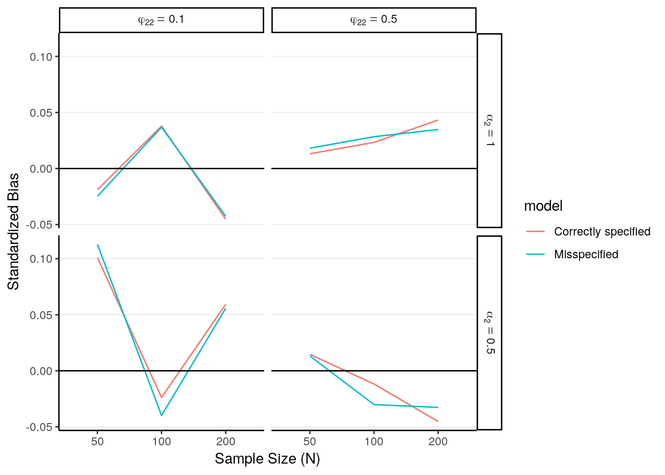
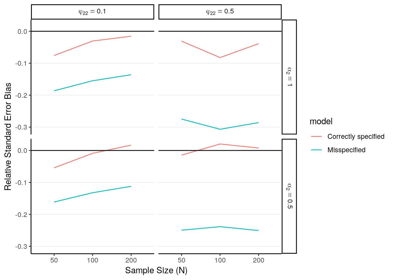
Finally, let’s summarize the results in terms of the standardized bias and the relative standard error bias.

sim_outdata <- sim_outdata %>% 
  # Make it long format
  gather("var", "val", m1_est:m2_se) %>% 
  separate(var, c("model", "var")) %>% 
  spread(var, val) %>% 
  # (Optional) Rename the levels of design factors to make it better looking in 
  # the plots
  mutate(model = factor(model, labels = c("Correctly specified", 
                                          "Misspecified")), 
         alpha2_lab = as_factor(paste0("alpha[2] == ", alpha2)), 
         phi22_lab = as_factor(paste0("phi[22] == ", phi22)), 
         N_lab = as_factor(paste0("italic(N) == ", N)))
sim_sum <- sim_outdata %>% 
  # Summarize results by conditions
  group_by(model, alpha2, phi22, N, alpha2_lab, phi22_lab, N_lab) %>% 
  summarise(ave_est = mean(est), 
            emp_sd = sd(est), 
            ave_se = mean(se)) %>% 
  # Compute standardized bias and relative SE bias
  mutate(bias = ave_est - alpha2, 
         bias_mcse = emp_sd / sqrt(NREP), 
         std_bias = bias / emp_sd, 
         rse_bias = (ave_se - emp_sd) / emp_sd) %>% 
  ungroup()

With relatively small number of conditions, one can present the results in a table (and it’s handy in R):

sim_sum %>% 
  select(model:N, 
         Bias = bias, `Monte Carlo Error` = bias_mcse, 
         `Standardized Bias` = std_bias, 
         `Relative SE Error` = rse_bias) %>% 
  knitr::kable(digits = 3L)

model	alpha2	phi22	N	Bias	Monte Carlo Error	Standardized Bias	Relative SE Error
Correctly specified	0.5	0.1	50	0.006	0.003	0.101	-0.054
Correctly specified	0.5	0.1	100	-0.001	0.002	-0.024	-0.009
Correctly specified	0.5	0.1	200	0.002	0.001	0.059	0.017
Correctly specified	0.5	0.5	50	0.002	0.005	0.015	-0.014
Correctly specified	0.5	0.5	100	-0.001	0.003	-0.012	0.020
Correctly specified	0.5	0.5	200	-0.002	0.002	-0.045	0.008
Correctly specified	1.0	0.1	50	-0.001	0.003	-0.019	-0.076
Correctly specified	1.0	0.1	100	0.002	0.002	0.038	-0.031
Correctly specified	1.0	0.1	200	-0.001	0.001	-0.045	-0.016
Correctly specified	1.0	0.5	50	0.001	0.005	0.013	-0.031
Correctly specified	1.0	0.5	100	0.002	0.004	0.023	-0.082
Correctly specified	1.0	0.5	200	0.002	0.003	0.043	-0.039
Misspecified	0.5	0.1	50	0.007	0.003	0.113	-0.161
Misspecified	0.5	0.1	100	-0.002	0.002	-0.040	-0.132
Misspecified	0.5	0.1	200	0.002	0.001	0.056	-0.112
Misspecified	0.5	0.5	50	0.001	0.005	0.013	-0.249
Misspecified	0.5	0.5	100	-0.002	0.003	-0.030	-0.238
Misspecified	0.5	0.5	200	-0.002	0.002	-0.033	-0.251
Misspecified	1.0	0.1	50	-0.002	0.003	-0.025	-0.186
Misspecified	1.0	0.1	100	0.002	0.002	0.037	-0.155
Misspecified	1.0	0.1	200	-0.001	0.001	-0.043	-0.136
Misspecified	1.0	0.5	50	0.002	0.005	0.018	-0.275
Misspecified	1.0	0.5	100	0.002	0.004	0.028	-0.307
Misspecified	1.0	0.5	200	0.002	0.003	0.035	-0.286

It is, however, recommended you try to plot the results, both for exploratory purpose and for better presentation of the results.

# Summarize estimates
sim_outdata %>% 
  ggplot(aes(x = factor(N), y = est, color = model)) + 
  geom_boxplot() + 
  geom_hline(aes(yintercept = alpha2)) + 
  facet_grid(alpha2_lab ~ phi22_lab, labeller = label_parsed) + 
  labs(x = "Sample Size (N)", y = "Estimates of Mean Slope")

# Standardized bias
sim_sum %>% 
  ggplot(aes(x = factor(N), y = std_bias, color = model)) + 
  geom_line(aes(group = model)) + 
  geom_hline(aes(yintercept = 0)) + 
  facet_grid(alpha2_lab ~ phi22_lab, labeller = label_parsed) + 
  labs(x = "Sample Size (N)", y = "Standardized Bias")

# Relative SE bias
sim_sum %>% 
  ggplot(aes(x = factor(N), y = rse_bias, color = model)) + 
  geom_line(aes(group = model)) + 
  geom_hline(aes(yintercept = 0)) + 
  facet_grid(alpha2_lab ~ phi22_lab, labeller = label_parsed) + 
  labs(x = "Sample Size (N)", y = "Relative Standard Error Bias")

3.4 Using the `SimDesign` package

Recently, the SimDesign package was developed so that designing and running simulation studies can be more structured and organized. The package also provides some great features such as parallel computing, fail-safe stopping, gathering of error or warning messages, among others. Check out the paper by Sigal & Chalmers (2016) as well as the package vignettes (https://cran.r-project.org/web/packages/SimDesign/index.html) for more information. Below is the R code for running the latent growth example with their package. Try it yourself!

library(tidyverse)
library(SimDesign)
library(mnormt)
library(lavaan)

# Design factors:
DESIGNFACTOR <- expand.grid(
  N = c(50, 100, 200), 
  phi22 = c(0.1, 0.5), 
  alpha2 = c(0, 0.5)
)
# Add condition number:
DESIGNFACTOR <- rowid_to_column(DESIGNFACTOR, "cond")
DESIGNFACTOR

# Function for generating data:
gen_lgm_data <- function(condition, fixed_objects = NULL) {
  N <- condition$N
  phi22 <- condition$phi22
  alpha2 <- condition$alpha2
  alpha <- c(1, alpha2)
  Phi <- matrix(c(1, phi22 / 2,
                  phi22 / 2, phi22), nrow = 2)
  Lambda <- cbind(c(1, 1, 1, 1), 
                  c(0, 1, 2, 3))
  Theta <- diag(0.5, nrow = 4)
  # Generate latent factor scores
  eta <- rmnorm(N, mean = alpha, varcov = Phi)
  # Generate residuals:
  e <- rmnorm(N, varcov = Theta)
  # Compute outcome scores
  y <- tcrossprod(eta, Lambda) + e
  colnames(y) <- paste0("y", 1:4)
  # Make it a data frame
  as.data.frame(y)
}
# Test: generate data
# test_df <- gen_lgm_data(DESIGNFACTOR[1, ])

# lavaan syntax (to be passed through `fixed_objects`)
# True model
M1 <- 'i =~ 1*y1 + 1*y2 + 1*y3 + 1*y4
       s =~ 0*y1 + 1*y2 + 2*y3 + 3*y4
       i ~~ s'
# Model without random slopes
M2 <- 'i =~ 1*y1 + 1*y2 + 1*y3 + 1*y4
       s =~ 0*y1 + 1*y2 + 2*y3 + 3*y4
       s ~~ 0*i + 0*s'

# Analysis function
run_lgm <- function(condition, dat, fixed_objects = NULL) {
  # Run model 1
  m1_fit <- growth(fixed_objects$M1, data = dat)
  # Run model 2
  m2_fit <- growth(fixed_objects$M2, data = dat)
  # Extract parameter estimates and standard errors
  ret <- c(coef(m1_fit)["s~1"], 
           sqrt(vcov(m1_fit)["s~1", "s~1"]),
           coef(m2_fit)["s~1"], 
           sqrt(vcov(m2_fit)["s~1", "s~1"]))
  names(ret) <- c("m1_est", "m1_se", "m2_est", "m2_se")
  ret
}
# Test: run analyses for simulated data
# run_lgm(dat = test_df)

# Helper function for computing relative SE bias
rse_bias <- function(est_se, est) {
  est_se <- as.matrix(est_se)
  est <- as.matrix(est)
  est_se <- colMeans(est_se)
  emp_sd <- apply(est, 2L, sd)
  est_se / emp_sd - 1
}

# Evaluative function
evaluate_lgm <- function(condition, results, fixed_objects = NULL) {
  alpha2 <- condition$alpha2
  c(bias = bias(results[ , c(1, 3)], parameter = alpha2), 
    std_bias = bias(results[ , c(1, 3)], parameter = alpha2, 
                    type = "standardized"), 
    rmse = RMSE(results[ , c(1, 3)], parameter = alpha2), 
    rse_bias = rse_bias(results[ , c(2, 4)], results[ , c(1, 3)])
  )
}

# Put all together
sim_results <- runSimulation(DESIGNFACTOR, 
                             replications = 500, 
                             generate = gen_lgm_data, 
                             analyse = run_lgm, 
                             summarise = evaluate_lgm, 
                             fixed_objects = 
                               list(M1 = M1, M2 = M2))

# With parallel processing (4 cores in this example; uncomment the following to
# run)
# sim_results <- runSimulation(DESIGNFACTOR, 
#                              replications = 500, 
#                              generate = gen_lgm_data, 
#                              analyse = run_lgm, 
#                              summarise = evaluate_lgm, 
#                              packages = c("mnormt", "lavaan"), 
#                              parallel = TRUE, 
#                              ncores = 4L, 
#                              fixed_objects = 
#                                list(M1 = M1, M2 = M2))

3.5 Exercise

From the simulation results, evaluate the relative efficiency of the estimated average slope (i.e., \(\alpha_2\)) under model 2 relative to that under model 1.