Monte Carlo Simulation Examples
2019-05-25
Note 1 Simulating Means and Medians
# Load required packages
library(tidyverse)
theme_set(theme_classic() +
            theme(panel.grid.major.y = element_line(color = "grey92")))
1.1 Central Limit Theorem (CLT)
We know that, based on the CLT, under very general regularity conditions, when sample size is large, the sampling distribution of the sample mean will follow a normal distribution, with mean equals to the population mean, \(\mu\), and standard deviation (which is called the standard error in this case) equals the population SD divided by the square root of the fixed sample size. Let \(\bar X\) be the sample mean, then
\[\bar X \sim \mathcal{N}\left(\mu, \frac{\sigma^2}{N}\right)\]
1.1.1 Examining CLT with Simulation
Let’s imagine a \(\chi^2\) distribution with four degrees of freedom in the population.
\[X \sim \chi^2(4)\]
ggplot(tibble(x = c(0, 20)), aes(x = x)) +
  stat_function(fun = dchisq, args = list(df = 4)) +
  labs(y = "density")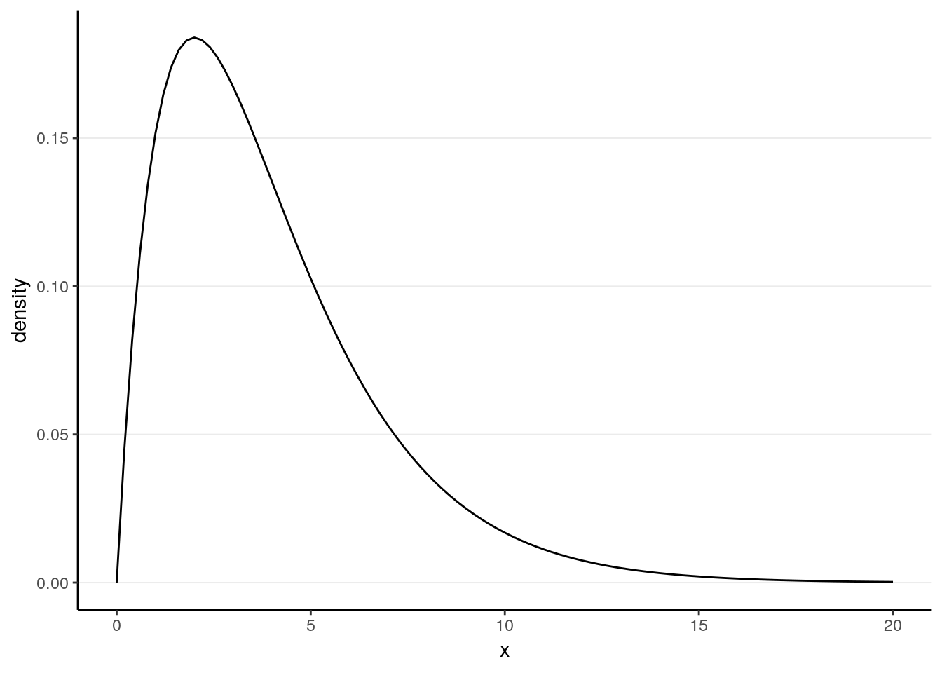
It is known that for a \(\chi^2(4)\) distribution, the population mean is \(\mu\) = 4 and the population variance is \(\sigma^2\) = \(2 \mu\) = 8, so we expect the mean of the sample means to be 4, and the standard error to be \(\sqrt{(8 / N)}\).
1.1.1.1 Sample size of 10
Let’s draw repeated samples of size 10 from this population. Here is the code
for doing it once, using the rchisq() function:
sample_size <- 10  # define sample size
sam1 <- rchisq(sample_size, df = 4)
mean(sam1)  # mean of the sample
># [1] 3.465038Now do it 1,000 times, using a for loop. Also, set the seed so that results are replicable:
NREP <- 1000  # number of replications
sample_size <- 10  # define sample size
# Initialize place holders for results
sam_means <- rep(NA, NREP)  # an empty vector with NREP elements
for (i in seq_len(NREP)) {
  sam_means[i] <- mean(rchisq(sample_size, df = 4))
}
# Plot the means:
ggplot(tibble(sam_means), aes(x = sam_means)) +
  geom_histogram()
># `stat_bin()` using `bins = 30`. Pick better value with `binwidth`.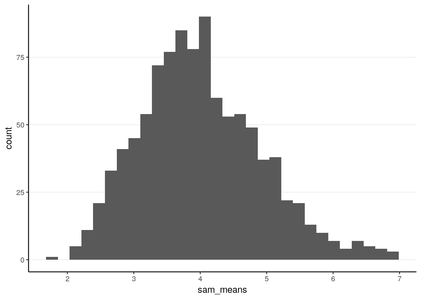
# Check normality
ggplot(tibble(sam_means), aes(sample = sam_means)) +
  stat_qq() +
  stat_qq_line()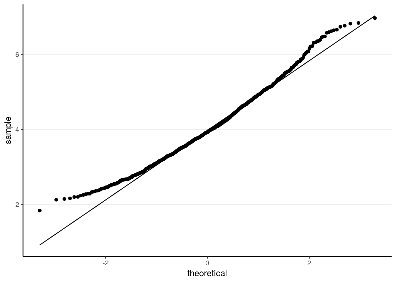
# Descriptive statistics
psych::describe(sam_means)
># vars n mean sd median trimmed mad min max range skew kurtosis
># X1 1 1000 4.01 0.91 3.92 3.96 0.91 1.84 6.97 5.13 0.48 0.09
># se
># X1 0.03As can be seen, it’s not fully normal. The mean of the sample means is 4.0070336, which is pretty close to the population mean of 4. The standard error is 0.9066569, also similar to the theoretical value.
1.1.1.2 Sample size of 50
Now, repeat the simulation with a sample size of 50
NREP <- 1000  # number of replications
sample_size <- 50  # define sample size
# Initialize place holders for results
sam_means <- rep(NA, NREP)  # an empty vector with NREP elements
for (i in seq_len(NREP)) {
  sam_means[i] <- mean(rchisq(sample_size, df = 4))
}
# Plot the means:
ggplot(tibble(sam_means), aes(x = sam_means)) +
  geom_histogram()
># `stat_bin()` using `bins = 30`. Pick better value with `binwidth`.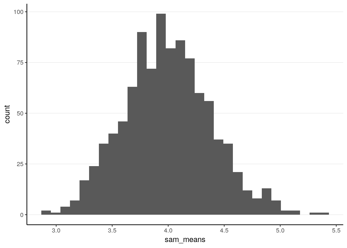
# Check normality
ggplot(tibble(sam_means), aes(sample = sam_means)) +
  stat_qq() +
  stat_qq_line()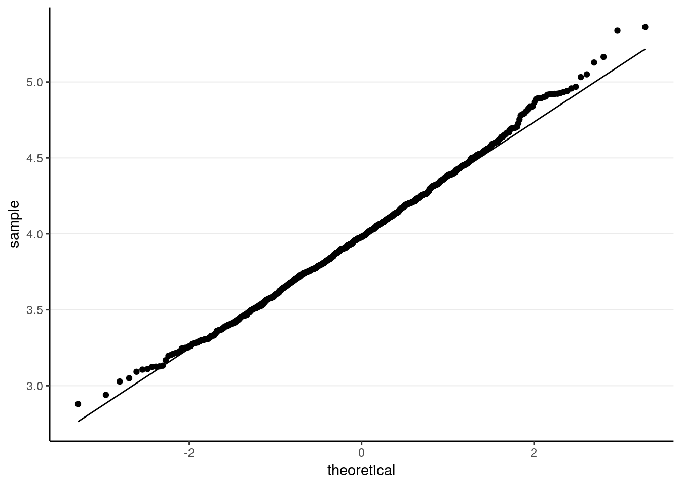
# Descriptive statistics
psych::describe(sam_means)
># vars n mean sd median trimmed mad min max range skew kurtosis
># X1 1 1000 3.99 0.39 3.98 3.99 0.37 2.88 5.36 2.48 0.2 0.04
># se
># X1 0.01The sampling distribution is closer to normal now. The standard error is of course smaller.
With these examples, hopefully you get an idea how simulation can be used to verify some theoretical results. Also, a lot of theoretical results only work for large samples, so simulation results fill the gap by providing properties of some estimators (sample mean of a \(\chi^2(4)\) distribution in this case) in finite samples.
1.2 Comparing Means and Medians
There is also a version of CLT for the sample medians, in that the median can also be used to estimate the population median. For symmetric distributions, this means that the sample median can also be used to estimate the population mean. Let’s try a normal distribution with mean of 4 and variance of 8:
NREP <- 1000  # number of replications
sample_size <- 10  # define sample size
# Initialize place holders for results
sam_medians <- rep(NA, NREP)  # an empty vector with NREP elements
for (i in seq_len(NREP)) {
  sam_medians[i] <- median(rnorm(sample_size, mean = 4, sd = sqrt(8)))
}
# Plot the means:
ggplot(tibble(sam_medians), aes(x = sam_medians)) +
  geom_histogram()
># `stat_bin()` using `bins = 30`. Pick better value with `binwidth`.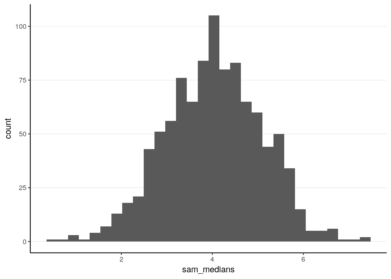
# Check normality
ggplot(tibble(sam_medians), aes(sample = sam_medians)) +
  stat_qq() +
  stat_qq_line()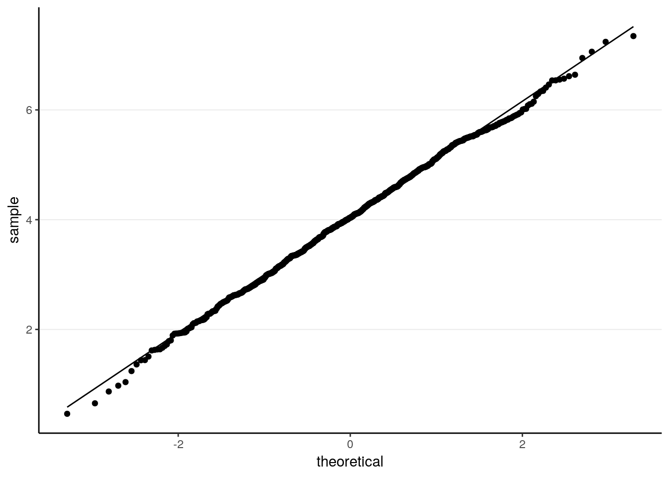
# Descriptive statistics
psych::describe(sam_medians)
># vars n mean sd median trimmed mad min max range skew kurtosis
># X1 1 1000 4.03 1.06 4.04 4.04 1.06 0.46 7.35 6.88 -0.09 -0.05
># se
># X1 0.03As can be seen, the sample median has a mean of 4.0321097, and a standard error of 1.0596777. Notably, this is larger than the theoretical standard error of the sample mean, 0.8944272.
1.2.1 Relative Efficiency
Thus, under the same sample size with a normal population, the standard error of the sample median is larger than that of the sample mean. This means that, on average, the sample mean will be closer to the population mean, even when both are unbiased. Therefore, the sample mean should be preferred, which is what we do.
When comparing two unbiased estimators, we say that the one with a smaller sampling variance (i.e., squared standard error) to be more efficient. The relative efficiency of estimator \(T_1\), relative to estimator \(T_2\), is defined as
\[\frac{\textrm{Var}(T_2)}{\textrm{Var}(T_1)}\] For example, based on our simulation results, the relative efficiency of the sample median, relative to the sample mean, is
var_sam_mean <- 8 / 10  # theoretical value
var_sam_median <- var(sam_medians)
(re_median_mean <- var_sam_mean / var_sam_median)
># [1] 0.7124303This means that in this case, the sample median is only 71% as efficient as the sample mean. Although it is true that for a normal distribution, the sample mean is more efficient than the sample median, there are situations where the sample median is more efficient. You can check that in the exercise.
1.2.2 Mean squared error (MSE)
The MSE is defined as the average squared distance from the sample estimator to the target quantity it estimates. we can obtain the MSE for the sample median in the previous example as:
(mse_sam_median <- mean((sam_medians - 4)^2))># [1] 1.122825In general, for any estimators \(T\) (with finite means and variances), the MSE can be decomposed as
\[\text{Bias}(T)^2 + \textrm{Var}(T)\]
so for unbiased estimators, MSE is the same as the sampling variance. On the other hand, for biased estimators, it is often of interest to compare their MSEs (or sometimes the square root of it, RMSE) to see which estimator has the best trade-off between biasedness and efficiency. Many estimators in statistics sacrifices a little bit in unbiasedness but get much smaller sampling variance.
1.3 Exercise
Generate a sample of 30 from a \(t\) distribution with df = 4. Show a plot of the data. Compute the sample mean and SD.
(Hint: you can use thert()function.)Compare the efficiency of the sample mean and the sample median in estimating the mean of a population following a student \(t\) distribution with df = 4. You can choose any sample size of at least 30. Which one, sample mean or sample median, is more efficient?