Note 2 Simulating Multilevel Data
# Load required packages
library(tidyverse)
theme_set(theme_classic() +
            theme(panel.grid.major.y = element_line(color = "grey92")))
library(mnormt)
library(lme4)
2.1 Linear Growth Model
General Mixed Model in Matrix form:
\[\begin{align*} Y_{ij} & = \boldsymbol{\mathbf{x}}_{ij} \boldsymbol{\mathbf{\beta}}_{j} + e_{ij} \\ \boldsymbol{\mathbf{\beta}}_{j} & = \boldsymbol{\mathbf{\gamma }}+ \boldsymbol{\mathbf{u}}_j, \end{align*}\]
with distributional assumptions:
\[\begin{align*} e_{ij} & \sim \mathcal{N}(0, \sigma^2) \\ \boldsymbol{\mathbf{u}}_{j} & \sim \mathcal{N}(\boldsymbol{\mathbf{0}}, \boldsymbol{\mathbf{G}}) \end{align*}\]
In a linear growth model, the predictor is time, and it’s assumed that
everyone in the data is measured with the same number of time points. A random
slope is included, meaning that the growth rates are different across
individuals. The two random effects, \(u_0\) (random intercepts) and \(u_1\) (random
slopes), have a variance-covariance matrix of \(\boldsymbol{\mathbf{G}}\) such that:
\[\begin{equation} \boldsymbol{\mathbf{G}} = \textrm{Var}(u_{j}) = \textrm{Var}\left(\begin{bmatrix} u_{0j} \\ u_{1j} \end{bmatrix}\right) = \begin{bmatrix} \tau_{00} & \tau_{01} \\ \tau_{01} & \tau_{11} \end{bmatrix}. \end{equation}\]
We’ll look into each step for simulating the data. For now, check out an example simulated data set first:
set.seed(2208)  # set the seed
J <- 20  # number of individuals (clusters)
cs <- 4  # number of time points (cluster size)
gam <- c(0, 0.5)  # fixed effects
G <- matrix(c(0.25, 0,
              0, 0.125), nrow = 2)  # random effect variances (G-matrix)
sigma2 <- 1  # within-person variance (lv-1)
X <- cbind(1, seq_len(cs) - 1)  # for each individual
X <- X[rep(seq_len(cs), J), ]  # repeat each row cs times
pid <- seq_len(J)  # individual id
pid <- rep(pid, each = cs)  # repeat each ID cs times
# Generate person-level (lv-2) random effects
uj <- rmnorm(J, mean = rep(0, 2), varcov = G)
# Generate repeated-measure-level (lv-1) error term
eij <- rnorm(J * cs, sd = sqrt(sigma2))
# Compute beta_j's
betaj <- matrix(gam, nrow = J, ncol = 2, byrow = TRUE) + uj
# Compute outcome:
y <- rowSums(X * betaj[pid, ]) + eij
# Form a data frame
sim_dat1 <- tibble(y, time = X[ , 2], pid)
# Plot the data:
sim_dat1 %>%
ggplot(aes(x = time, y = y, color = factor(pid), group = pid)) +
geom_line() + # individual trajectory
geom_smooth(aes(group = 1), method = "lm") # overall trend line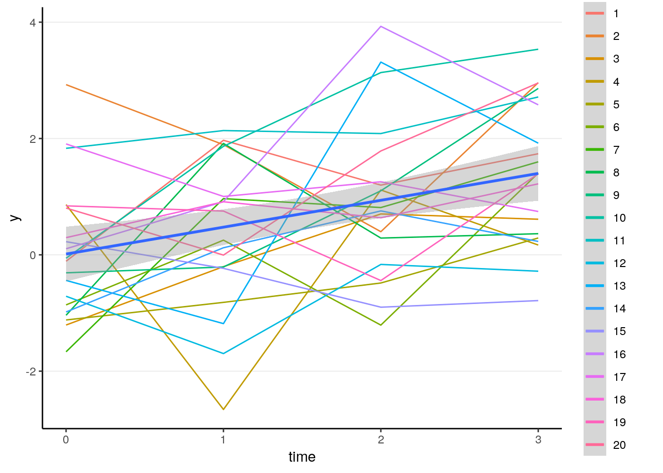
# Run multilevel model:
summary(lmer(y ~ time + (time | pid), data = sim_dat1))
># Warning in checkConv(attr(opt, "derivs"), opt$par, ctrl =
># control$checkConv, : Model failed to converge with max|grad| = 0.00340355
># (tol = 0.002, component 1)># Linear mixed model fit by REML ['lmerMod']
># Formula: y ~ time + (time | pid)
># Data: sim_dat1
>#
># REML criterion at convergence: 254.2
>#
># Scaled residuals:
># Min 1Q Median 3Q Max
># -2.58337 -0.52403 0.00055 0.45941 2.26654
>#
># Random effects:
># Groups Name Variance Std.Dev. Corr
># pid (Intercept) 0.33239 0.5765
># time 0.02529 0.1590 0.70
># Residual 0.99704 0.9985
># Number of obs: 80, groups: pid, 20
>#
># Fixed effects:
># Estimate Std. Error t value
># (Intercept) 0.01368 0.22697 0.060
># time 0.46195 0.10600 4.358
>#
># Correlation of Fixed Effects:
># (Intr)
># time -0.489
># convergence code: 0
># Model failed to converge with max|grad| = 0.00340355 (tol = 0.002, component 1)2.1.1 Overview of Simulation Process for Linear Growth Model
- Set the seed
set.seed(2208) # set the seed- Define Simulation Parameters:
The parameters are:
- Number of individuals/clusters (
J) - Number of time points (cluster size,
cs) - Fixed effects (
gam):- \(\gamma_0\) = grand intercept
- \(\gamma_1\) = average slope
- Variance-covariance matrix of random effects (
Gmatrix)- There are two random effects, so a 2 x 2 matrix
- Within-person error variance (\(\sigma^2\),
sigma2)
J <- 20  # number of individuals (clusters)
cs <- 4  # number of time points (cluster size)
gam <- c(0, 0.5)  # fixed effects
G <- matrix(c(0.25, 0,
              0, 0.125), nrow = 2)  # random effect variances (G-matrix)
sigma2 <- 1 # within-person variance (lv-1)- Define the design matrix (i.e., predictor matrix)
X <- cbind(1, seq_len(cs) - 1)  # for each individual
X <- X[rep(seq_len(cs), J), ] # repeat each row cs times- Generating ID variable
pid <- seq_len(J)  # individual id
pid <- rep(pid, each = cs) # repeat each ID cs times- Simulating random components
In this example, the three random components are: \(u_{0j}\), \(u_{1j}\), and
\(e_{ij}\). \(u_{0j}\) and \(u_{1j}\) are multivariate normal, each of length J, and
\(e_{ij}\) is normal of length J * cs.
# Generate person-level (lv-2) random effects
uj <- rmnorm(J, mean = rep(0, 2), varcov = G)
# Generate repeated-measure-level (lv-1) error term
eij <- rnorm(J * cs, sd = sqrt(sigma2))
6a. Compute \(\beta\)s
# Compute beta_j's
betaj <- matrix(gam, nrow = J, ncol = 2, byrow = TRUE) + uj
6b. Compute \(y\)s
# Compute outcome:
y <- rowSums(X * betaj[pid, ]) + eij- Combine into a data frame
# Form a data frame
sim_dat1 <- tibble(y, time = X[ , 2], pid)
2.1.2 Define a Data Generating Function
Because the data generating process will be repeated numerous time, it is beneficial to make it into a function. There are, however, some decisions to be made regarding which part of the simulation should go into a function, and which part(s) should become the arguments of the function. For example, I can set a function that create the number of clusters, cluster sizes, and everything inside the function, and the function basically just rerun steps 1 to 7. Such a function, however, will not be very useful as it is likely that one may want to change these parameters to be different in various simulation conditions. In this example, I have decided to create a function that has the following arguments (parameters):
J,cs,gam,G,sigma2
I will treat X as the same, meaning that the simulation function likely will
be only used for generating data with linear growth. If other growth shape will
be compared in the simulation study, then it may be better to include X as an
argument of the function so that it’s easier to change it.
After all, the fewer parameters there are in a function, the more specific the function is; the more parameters, the more general it is. There should be a balance between the two.
Okay, here is the function:
gen_lg_data <- function(J, cs, gam, G, sigma2 = 1) {
  X <- cbind(1, seq_len(cs) - 1)  # for each individual
  X <- X[rep(seq_len(cs), J), ]  # repeat each row cs times
  pid <- seq_len(J)  # individual id
  pid <- rep(pid, each = cs)  # repeat each ID cs times
  # Generate person-level (lv-2) random effects
  uj <- rmnorm(J, mean = rep(0, 2), varcov = G)
  # Generate repeated-measure-level (lv-1) error term
  eij <- rnorm(J * cs, sd = sqrt(sigma2))
  # Compute beta_j's
  betaj <- matrix(gam, nrow = J, ncol = 2, byrow = TRUE) + uj
  # Compute outcome:
  y <- rowSums(X * betaj[pid, ]) + eij
  # Form a data frame
  sim_dat1 <- tibble(y, time = X[ , 2], pid)
  # Return data
  return(sim_dat1)
}
I can generate some data with 30 people and 4 time points:
gen_lg_data(30, 4, gam = c(0, 0.5),
            G = matrix(c(0.1, 0,
                         0, 0.01), nrow = 2))  # sigma2 is default to 1.0
># # A tibble: 120 x 3
># y time pid
># <dbl> <dbl> <int>
># 1 1.60 0 1
># 2 0.0834 1 1
># 3 1.21 2 1
># 4 2.37 3 1
># 5 -0.386 0 2
># 6 -0.276 1 2
># 7 0.298 2 2
># 8 0.443 3 2
># 9 -0.0782 0 3
># 10 -0.0982 1 3
># # … with 110 more rowsNote that I set the default of sigma2 to 1 as this can be constant across
conditions. This is useful for a parameter that are mostly constant, but I just
want to make the function work in case I need the parameter to be something
different.
I can generate with 50 people and 6 time points:
gen_lg_data(50, 6, gam = c(0, 0.5),
            G = matrix(c(0.1, 0,
                         0, 0.01), nrow = 2))  # sigma2 is default to 1.0
># # A tibble: 300 x 3
># y time pid
># <dbl> <dbl> <int>
># 1 1.54 0 1
># 2 1.34 1 1
># 3 1.91 2 1
># 4 0.978 3 1
># 5 2.04 4 1
># 6 2.02 5 1
># 7 0.128 0 2
># 8 -0.393 1 2
># 9 0.457 2 2
># 10 0.140 3 2
># # … with 290 more rows2.1.3 Define a Function to Run the Analysis
I just realized I haven’t told you the goal of the simulation. Let’s say I’m interested in what will happen to the fixed effect estimates when the random slope term is ignored. To do that, for each generated data set, I need to fit a multilevel model ignoring the random slope. Here’s a function to do that:
# Function to run a random intercept model
run_ri <- function(df) {
  # Only requires input of a data frame
  lmer(y ~ time + (1 | pid), data = df)
}
# Test it on our simulated data set:
run_ri(sim_dat1)
># Linear mixed model fit by REML ['lmerMod']
># Formula: y ~ time + (1 | pid)
># Data: df
># REML criterion at convergence: 255.329
># Random effects:
># Groups Name Std.Dev.
># pid (Intercept) 0.7554
># Residual 1.0187
># Number of obs: 80, groups: pid, 20
># Fixed Effects:
># (Intercept) time
># 0.01368 0.461952.1.4 Run the Simulation
Now, we can create a for loop to run the simulation:
# Set the seed
set.seed(2208)
# Note: use capital letters for GLOBAL VARIABLES
NREP <- 100  # number of replications; should be increased in practice
J <- 20  # number of individuals (clusters)
CS <- 4  # number of time points (cluster size)
GAM <- c(0, 0.5)  # fixed effects
G <- matrix(c(0.25, 0,
              0, 0.125), nrow = 2)  # random effect variances (G-matrix)
# Initialize place holders for results
sim_result <- vector("list", length = NREP)
# Create a for loop:
for (i in seq_len(NREP)) {
  sim_dat <- gen_lg_data(J, CS, GAM, G)
  sim_result[[i]] <- run_ri(sim_dat)
}
# Check the last result:
sim_result[[NREP]]
># Linear mixed model fit by REML ['lmerMod']
># Formula: y ~ time + (1 | pid)
># Data: df
># REML criterion at convergence: 264.3811
># Random effects:
># Groups Name Std.Dev.
># pid (Intercept) 0.6601
># Residual 1.1184
># Number of obs: 80, groups: pid, 20
># Fixed Effects:
># (Intercept) time
># -0.2072 0.67482.1.5 Extract Target Statistics
Let’s extract the fixed effect for the time variable for each result. We can use
the purrr::map() function (or you can do a for loop too):
# The `fixef` function can extract the fixed effect coefficients
fixef(sim_result[[1]])
># (Intercept) time
># 0.01367995 0.46194936# The following extracts the standard error
sqrt(diag(vcov(sim_result[[1]])))># [1] 0.2546643 0.1018698# And confidence intervals:
confint(sim_result[[1]], parm = "time")># 2.5 % 97.5 %
># time 0.2607471 0.6631516# Now get the fixed effect and the standard error for all replications
fixefs_time <- map(sim_result,
~ tibble(est = fixef(.x)[2],
se = sqrt(diag(vcov(.x))[2]),
ci = confint(.x, parm = "time")) %>%
# expand CI to two columns
transmute(est, se, li = ci[1], ui = ci[2])) %>%
# merge the results
bind_rows()2.1.6 Summarize the Results
We can plot the sampling distribution of the fixed effect coefficient
fixefs_time %>%
  ggplot(aes(x = est)) +
  geom_density()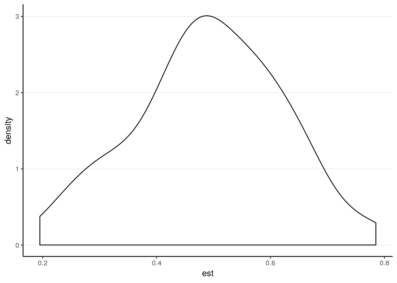
The main evaluation is the bias and SE bias:
# bias:
summarize(fixefs_time,
          ave_est = mean(est),
          ave_se = mean(se),
          sd_est = sd(est),
          ci_coverage = mean(li <= GAM[2] & ui >= GAM[2])) %>%
  # Compute bias and SE bias
  mutate(bias = ave_est - GAM[2],
         rbias = bias / GAM[2],
         se_bias = ave_se - sd_est,
         rse_bias = se_bias / sd_est,
         rmse = bias^2 + sd_est^2)
># # A tibble: 1 x 9
># ave_est ave_se sd_est ci_coverage bias rbias se_bias rse_bias
># <dbl> <dbl> <dbl> <dbl> <dbl> <dbl> <dbl> <dbl>
># 1 0.492 0.110 0.129 0.86 -0.00826 -0.0165 -0.0191 -0.149
># # … with 1 more variable: rmse <dbl>2.2 Exercise
Create a new function,
run_rs(), which analyze the data with the random slope term, by modifying therun_ri()function.Replicate the previous simulation, but with the new function.
Compare the results with and without random slopes.