Section 2 Tips for effective R programming
Before getting into actual R code, we’ll start with a few notes about how to use it most effectively. Bad coding habits can make your R code difficult to read and understand, so hopefully these tips will ensure you have good habits right from the start.
2.1 Use RStudio’s “projects” feature
Every project you do in R should be set up in its own folder, through RStudio’s “projects” feature. To start a fresh project, go to File -> New project and create a new folder. Reopen the project in RStudio whenever you want to work with it.
When sending your work to other people, you can send them the whole folder and know that they’ll have access to all the required files and scripts.
One of the main benefits is that this sets R’s “working directory” to the project folder by default. Any files you load or save can just be referenced relative to that folder, so instead of:
You can just do:
This will also work for anyone you send the project to, so you don’t have to worry that the file is in a different location on their machine.
2.2 Using scripts
It’s best to put every step of your data cleaning and analysis in a script that you save, rather than making temporary changes in the console.
Ideally, this will mean that you (or anyone else) can run the script from top to bottom, and get the same results every time, i.e. they’re reproducible.
2.2.1 Script layout
Most R scripts I write have the same basic layout:
- Loading the libraries I’m using
- Loading the data
- Changing or analysing the data
- Saving the results or the recoded data file
For a larger project, it’s good to create multiple different scripts for each stage, e.g. one file to recode the data, one to run the analyses.
When saving the recoded data, it’s best to save it as a different file - you keep the raw data, and you can recreate the recoded data exactly by rerunning your script.
R won’t overwrite your data files when you change your data, unless you specifically ask it to. When you load a file into R, it lives in R’s ‘short-term memory’, and doesn’t maintain any connection to the file on disk. It’s only when you explicitly save to a file that those changes become permanent.
2.2.2 A tip for better reproducibility
By default, RStudio will save your current “workspace” when you quit. While convenient, this can mean that you make one-off changes to your data and forget to save that command in your script. Starting with a fresh session every time you open RStudio means you’ll learn to keep every step of your analysis in your script, and you’ll know that you can get back to where you were by rerunning the script.
To disable the default setting, go to Tools -> Global options.., and in the General tab, and:
- Uncheck “Restore .RData”
- Set “Save workspace on exit” to “Never”
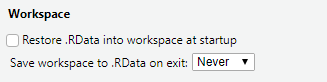
RStudio’s “save workspace” settings
2.3 Long or wide data
R works better with long data, whereas SPSS generally works better with wide data. Roughly speaking, long data means:
- There is one “observation” of each participant/subject per row - e.g. one survey, one session
- All the measurements of the same type are in one column - so all the
K6 scores, from multiple surveys, would be in a single
K6column, with an additionalTimeorSurveycolumn that identifies which survey they come from.
Example long data:
| ID | Survey | Drinking | AnxietyTotal |
|---|---|---|---|
| 1 | 1 | No | 6 |
| 1 | 2 | Yes | 8 |
| 2 | 1 | No | 5 |
| 2 | 2 | No | 7 |
Example wide data:
| ID | Drinking_T1 | Drinking_T2 | AnxietyTotal_T1 | AnxietyTotal_T2 |
|---|---|---|---|---|
| 1 | No | Yes | 6 | 8 |
| 2 | No | No | 5 | 7 |
2.3.1 Going from wide to long
If your data is currently in wide format, you may have to reshape
it before working with it in R. The new pivot_longer and pivot_wider
functions from the tidyr package are good for reshaping data like this.
To go from the wide data above to a long dataset:
wide %>%
    tidyr::pivot_longer(
        cols = Drinking_T1:AnxietyTotal_T2,
        names_to = c(".value", "Time"),
        names_sep = "_"
    )
This can get more complicated if the columns haven’t been
named consistently, or have multiple pieces of info
stored in the name (e.g. t1_male_mean)
At the time of writing, the pivot functions were still in beta, but should be in the new tidyr version shortly.
2.4 Writing readable code
There are two very good reasons to try to write your code in a clear, understandable way:
- Other people might need to use your code.
- You might need to use your code, a few weeks/months/years after you’ve written it.
It’s possible to write R code that “works” perfectly, and produces all the results and output you want, but proves very difficult to make changes to when you have to come back to it (because a reviewer asked for one additional analysis, etc.)
2.4.1 Basic formatting tips
You can improve the readability of your code a lot by following a few simple rules:
- Put spaces between and around variable names and operators (
=+-*/) - Break up long lines of code
- Use meaningful variable names composed of 2 or 3 words (avoid abbreviations unless they’re very common and you use them very consistently)
These rules can mean the difference between this:
and this:
male_difference = lm(DepressionScore ~ Group + GroupTimeInteraction,
                     data = interview_data,
                     subset = BaselineSex == "Male")
R will treat both pieces of code exactly the same, but for any humans reading, the nicer layout and meaningful names make it much easier to understand what’s happening, and spot any errors in syntax or intent.
2.4.2 Keeping a consistent style
Try to follow a consistent style for naming things, e.g. using snake_case
for all your variable names in your R code, and TitleCase for the
columns in your data. Either style is probably better than lowercase with
no spacing allmashedtogether.
It doesn’t particularly matter what that style is, as long as you’re consistent. There is a suggested style guide for the tidyverse, but I don’t follow it 100%, I just try to be consistent within my code.
2.4.3 Writing comments
One of the best things you can do to make R code readable and
understandable is write comments - R ignores lines that start with
# so you can write whatever you want and it won’t affect
the way your code runs.
Comments that explain why something was done are great:
Comments that explain what is being done are less useful. People who already understand R code should be able to tell what is happening just by looking at your code (especially if you’re following the other advice about writing readable code), so these comments can be redundant:
The exception to this is when you’ve run into something that was tricky to get working, and you need to explain it so other people don’t run into the same issue:
2.5 Don’t panic: dealing with SPSS withdrawal
2.5.1 RStudio has a data viewer
As you get used to R, you should find that you get more comfortable
using the console to check on your data. You can often see
a lot of the information you need by printing the first few
rows of a dataset to the console. The head() function prints
the first 6 rows of a table by default, and you can select the columns that
are most relevant to what you’re working on if there are too many:
##   Species Petal.Length
## 1  setosa          1.4
## 2  setosa          1.4
## 3  setosa          1.3
## 4  setosa          1.5
## 5  setosa          1.4
## 6  setosa          1.7
However, you can also use RStudio’s built-in data viewer to get a more familiar, spreadsheet style view of your data. In the Environment pane in the top-right, you can click on the name of any data you have loaded to bring up a spreadsheet view:
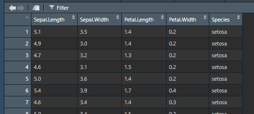
Data viewer example
This also supports basic sorting and filtering so you can explore
the data more easily (you’ll still need to write code using functions
like arrange() or filter() if you want to actually make
changes to the data though).
2.5.2 R can read SPSS files
The haven package can read (and write) SPSS data files, so you
can read in existing data:
R doesn’t deal with “value labels” in the same way as SPSS, and
haven tries to keep information about the SPSS value labels available.
However, it’s best to just convert everything to R’s way of dealing with
categorical variables, i.e. factors, using haven’s as_factor() function:
The levels = "both" option puts both the numeric value and the text label
into the factor labels, like "[0] No", "[1] Yes". As you get more
comfortable with R you may want to just use levels = "labels" so you
just get the text labels like "No", "Yes".
You may need to convert your data from wide to long, since SPSS prefers wide and R prefers long.
The haven package can also read SAS and Stata data, and there are
packages like readxl for Excel files. It’s generally easy to read
your data into R from any format designed for tables of data.
2.6 Here be dragons: the bad parts of R
There are a few tools in R that tend to create more problems than they solve. Unfortunately beginners often end up using them (sometimes because bad tutorials recommend them). My personal list of tools to avoid includes:
attach(): This copies all the individual variables from a dataset into R’s environment, so you can access them with justvar_nameinstead ofdataset$var_name. The problem is:- You end up with a lot of variables in your environment that are hard to keep track of.
- The variables can get out of sync with each other in ways that wouldn’t be possible if they were kept in the dataset.
get()andassign(): These allow you to look up and create variable names using strings, so instead of looking upmodel3, you can programmatically create the variable name likeget(paste0("model", model_num)).- Again, you can end up with a lot of variables in your environment.
- People often use these when they want to run 100 different versions
of a model (there are sometimes good reasons to do this). Instead of creating
100 different variables called
model1,model2, …,model100, it’s usually possible to save these in a singlelistor dataframe. Saving them all in a list means it’s much easier to process and work with the results.