9 Advanced Methods
9.1 Create an Account at the UCSC Genome Browser
Creating an account at the UCSC Genome Browser site is useful for a variety of reasons. For example, having an account will enable you to save your favorite settings into a named session, and then return to the named session later regardless of which computer you use. You can also share named sessions with other users (something I will do for you throughout the semester).
To create an account, go to the UCSC Genome Browser. In the toolbar at the top of the page hover over “My Data” then choose “My Sessions” from the pulldown menu. At the top of the page click “Create an Account”. Complete the form then click “Sign Up”. You are done!
9.2 How to Configure the Genome Browser from Scratch
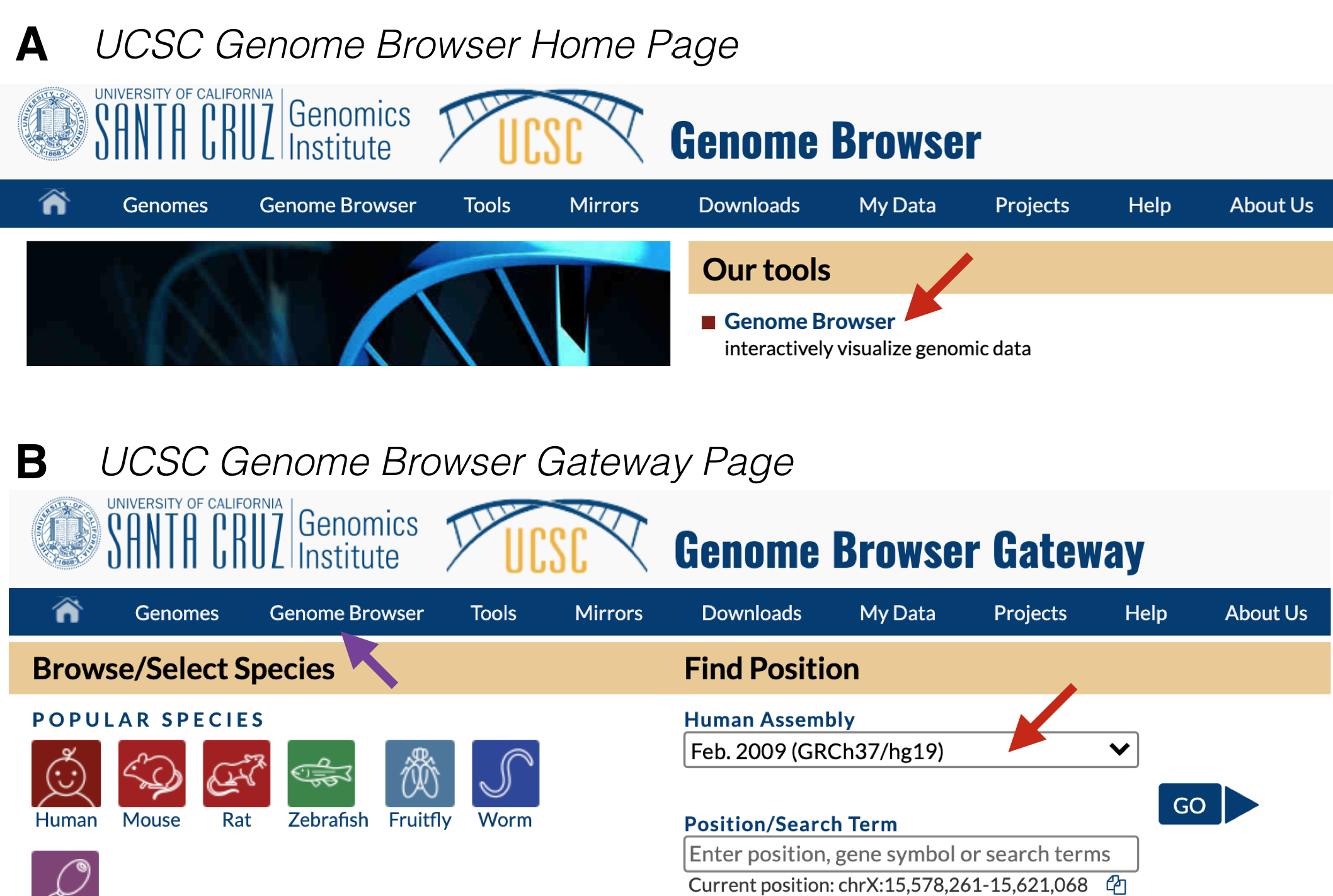
Figure 9.1: A) This is the UCSC Genome Browser Homepage. Click on Genome Browser (red arrow) to get to the Browser Gateway Page. B) This is the Browser Gateway Page. Choose the Feb. 2009 Human assembly (red arrow) then click Go.
To begin from scratch, go to the UCSC Genome Browser. At the home page, click on “Genome Browser” under “Our Tools” (Figure 9.1 A). Within the Genome Browser Gateway page, hover your mouse over “Genome Browser” in the tool bar (Figure 9.1 B, purple arrow) and click on “Reset All User Settings”. Then click on the pull down menu under Human Assembly77 and choose “Feb. 2009 (GRCh37/hg19)” (Figure 9.1 B, red arrow). Now click “Go” to be taken to the Human Genome Browser window.
Since you did not search for a specific gene, you have been taken to a default position within the genome, specifically, a small region on the short arm of the X chromosome where a gene called ACE2 resides (Figure 9.2 A and B). Why here? This paragraph was written in 2020 when ACE2 became infamous. Google “ACE2” and “coronavirus” to see why!
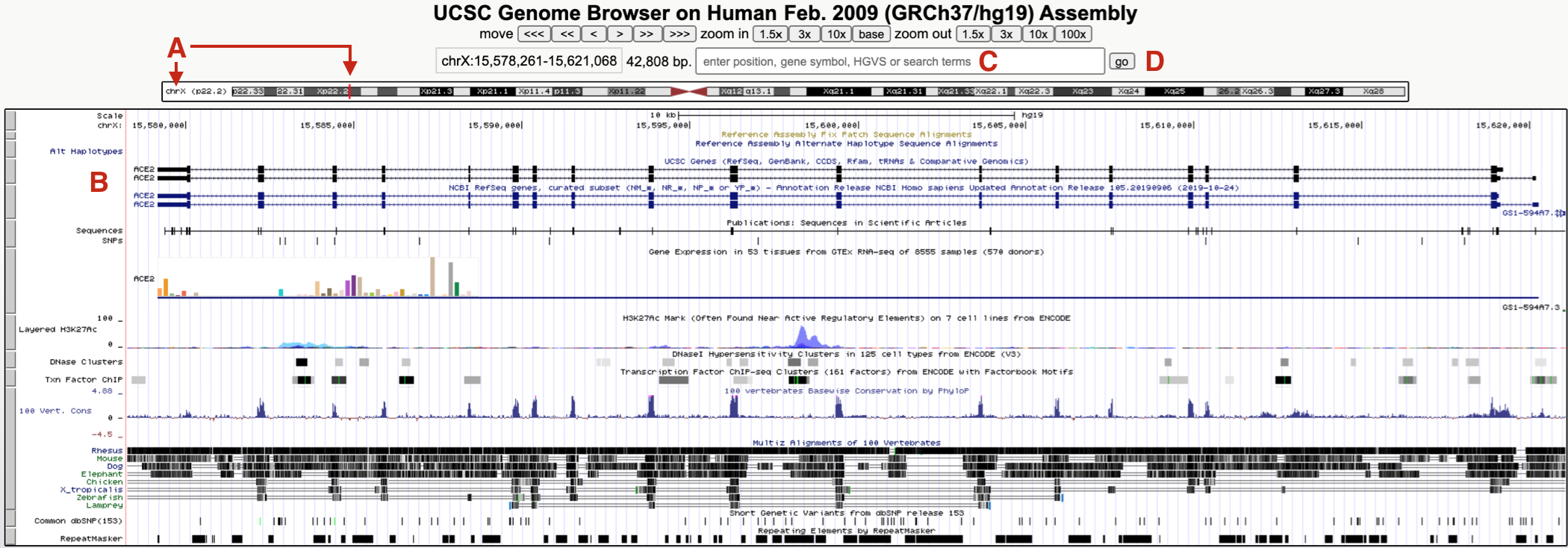
Figure 9.2: The UCSC Genome Browser window focused on a small region of the X chromosome (A) on a gene called ACE2 (B). To hop to BBS1, use the search window (C) then click Go (D). See text for important details.
To hop to where BBS1 resides, type BBS1 into the search window (Figure 9.2 C). As you type, a popup menu will appear with a short list of related genes. Choose BBS1 then click “GO” (Figure 9.2 D). If you do not choose a gene from this list, you will be transported to a new page with a long list of related genes grouped according to sequence database (there are many). It might be easiest to go back and try again. Alternatively, scroll down until you find the “NCBI RefSeq” database78 then click on the link for BBS1.
Your browser window should now jump to chromosome 11 (Figure 9.3 A). The default genome browser window will now display a variety of so-called “evidence tracks”. These are graphical representations of genome features or experimental data related to the region displayed. Nearly all evidence tracks include a centrally located title heading (Figure 9.3 B) and all include a gray rectangle positioned on the left (Figure 9.3 C). Three evidence tracks are highlighted in total. The one at the top is the Base Position track (Figure 9.3 D). This is the only evidence track that does not have a track title. This track displays the genome sequence itself. That said, you will only be able to see individual nucleotides when you zoom in close enough. Two Gene Prediction tracks are also highlighted. One is the “UCSC Genes” track (Figure 9.3 E). Another is the “NCBI Refseq genes” track (Figure 9.3 C). Notice the gene name is displayed on the left side of each schematic.
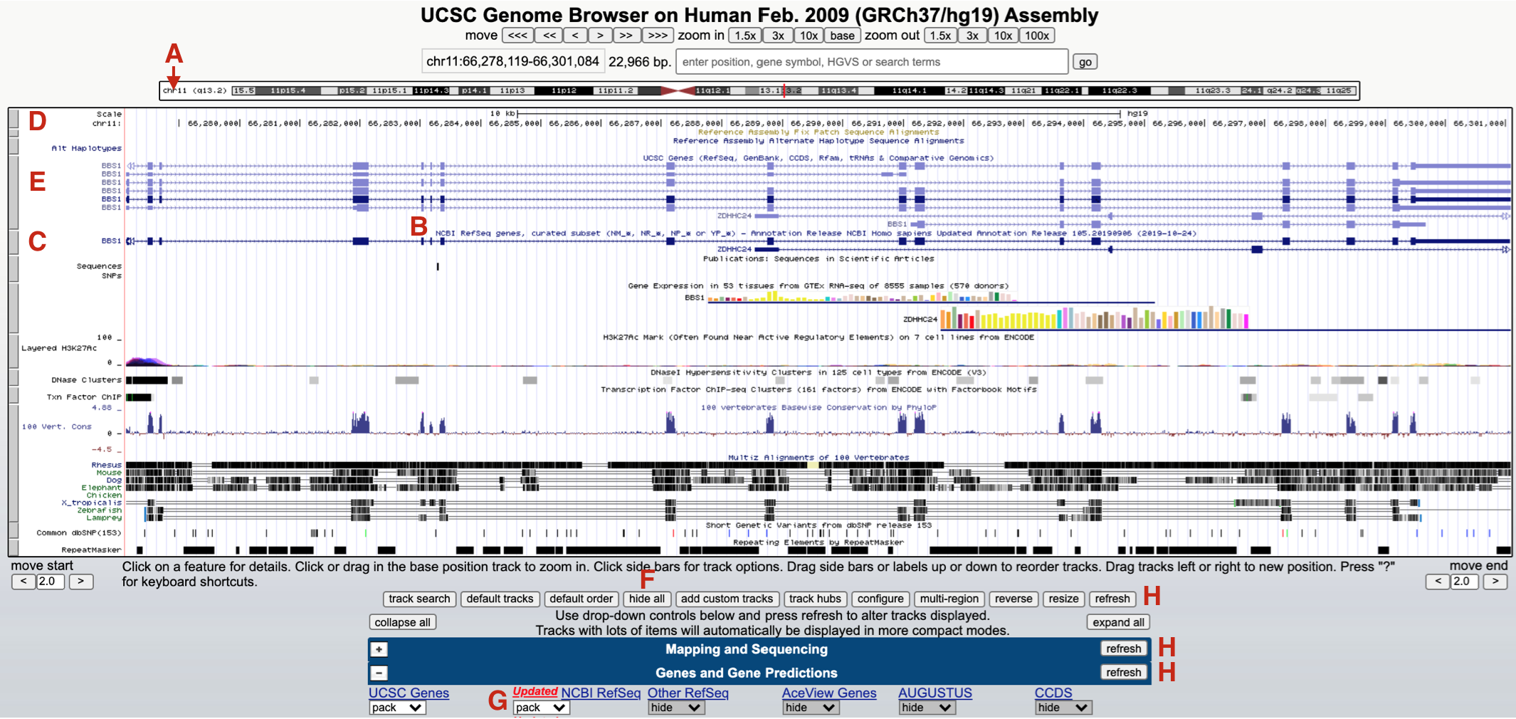
Figure 9.3: The browser window now focused on a small region of chromosome 11 (A) where BBS1 resides (C and E). Each evidence track includes a track title (B) and is demarcated by a gray rectangle (D, E and C). To hide all tracks click hide all (F) and click refresh (H). To open the NCBI Refseq track change the pulldown menu from hide to pack (G).
Each gray rectangle corresponding to an evidence track is clickable. Clicking on a gray rectangle will take you to a track settings page for that particular evidence track. Try it. Then click the back button to get back. Right clicking on a gray rectangle on the other hand will open up a small window for quick formatting. For example, you can hide any evidence track that you don’t need in this way. To hide all evidence tracks at once, scroll down to below the browser window and click “hide all” (Figure 9.3 F). Everything but the Base Position track will disappear. Now scroll down to view the most commonly used evidence tracks below the browser window to confirm. All but the “Base Position” track found within the “Mapping and Sequencing” section should be set to hide. Now change the “NCBI Refseq” evidence track (found within the “Genes and Gene Predictions” section) to “pack” (Figure 9.3 G) and click “refresh” (Figure 9.3 H). You should now see only two gray rectangles on the left. The base position track on top and the “NCBI refseq genes” Gene Prediction track is below (Figure 9.4).
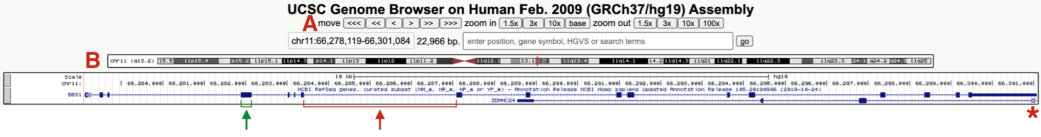
Figure 9.4: This is what the BBS1 Gene Structure named session should look like. One example of an exon and intron are highlighted. The asterix points on the right highlights the open triangles extending from ZDHHC24 indicating that this gene extends further to the right. (A) highlights the navigational toolbar and (B) highights the schematic of the chromosome where BBS1 resides. One exon (green bracket) and one intron (red bracket) are also shown.
Again, the “NCBI Refseq genes” evidence track includes a graphical representation of the BBS1 gene79. This gene schematic displays the position of BBS1 exons and introns (see red and green brackets in Figure 9.4). You may also notice that a second gene (ZDHHC24) partly overlaps BBS1. The open arrowheads at the far right of the graphical representation for ZDHHC24 (red asterisk, Figure 9.4) indicates that this gene extends farther to the right.
9.3 Creating a Named Session
Compare what you configured to my named session, BBS1 gene structure. If they are identical, congratulations. If not, try again but don’t stress too much. You can always use my link to get to a correctly formatted page. You are now ready to create your own named session based on the browser window you created (or mine). First, make sure your browser window looks the way you want it to. Next, make sure you are logged into your account. Hover your mouse over “My Data” then click on “My Sessions”. Scroll down to the section entitled, “Save Settings”. Within the window under “Save current settings as named session”, input a reasonable name for this session (i.e. “Gene and Base Prediction Tracks only”). Then hit submit. Now anytime you want to sit down at a computer (anywhere, any computer) to view BBS1 with only the base position and gene prediction tracks open, you simply need to log into your UCSC Genome Browser account, go into “My Sessions” and click on your named session. You won’t need to rely on this manual for links. You can also use this named session as a springboard to view any other gene by using the search window.
© 2019, Maria Gallegos. All rights reserved.
pleiotropy is a condition in which a single gene influences more than one trait (Snustad).↩︎
a chromosome is a single, long molecule of DNA↩︎
Many organisms are diploid (including humans) meaning they have two copies of each chromosome. Thus the phrase “haploid genome” is more precise, although the word “haploid” is often omitted and simply assumed↩︎
One way to calculate the length of a chromosome: Multiply the length of a chromosome in base pairs (bp) with 0.000000332, the length (in mm) of each bp.↩︎
Cells of a multicellular organism can be divided into two main types: germ cells and somatic cells. Germ cells are destined to become the reproductive cells like sperm and oocytes. Somatic cells are destined to become all the other cell types like skin, neurons and muscle. This distinction is made as somatic cells die with the death of the organism while germ cells have the potential to pass their DNA on to the next generation.↩︎
An autosome is one of the numbered chromosomes, as opposed to the sex chromosomes. Autosomes are numbered roughly in relation to their sizes. The largest autosome — chromosome 1 — has approximately 2,800 genes; the smallest autosome — chromosome 22 — has approximately 750 genes. This definition is found at https://www.genome.gov/genetics-glossary/Autosome↩︎
a unit of length equal to one hundred-millionth of a centimeter - Definition from Oxford Languages↩︎
A “reference genome” (also called a “reference assembly”) is a genome sequence created from thousands of sequence runs assembled in silico to represent the sequence of a genome of one idealized individual organism. Since it is assembled from sequence data obtained from a number of donors, reference genomes do not represent the sequence of any single individual or organism, but rather a mosaic of multiple donors↩︎
each evidence track harbors specific biological data from a single source pertaining to the sequence displayed in the browser window)↩︎
The top strand of DNA is also referred to as the “+ strand”↩︎
A chain of amino acids linked together by peptide bonds. While the words “protein” and “polypeptide” are often used interchangeably, the term protein is more vague. It could refer to a single polypeptide or it might mean multiple polypeptides bound together in a complex. On the other hand, polypeptide always refers to a single sequence of amino acids↩︎
A cytoplasmic machine (comprised of RNA and protein) which uses the mRNA to synthesize a polypeptide.↩︎
A set of three adjacent nucleotides in an mRNA molecule that either specify the incorporation of an amino acid in a growing polypeptide chain or signals the end of polypeptide synthesis. Codons with the latter function are called termination codons (Snustad).↩︎
If you do not see the amino acid sequence displayed over the exon schematic, you may need to zoom in farther. If you are zoomed in enough to see the genome sequence, then something else is wrong. Instead, right click on the gray rectangle corresponding to the Gene Prediction track and choose, “Configure RefSeq Curated”. Then change “Color track by codons:” from “OFF” to “genomic codons”↩︎
used as the template for transcription and by definition is complementary to the top strand↩︎
Notice that at this zoom level some exons simply look like vertical lines. This is because, exons are typically shorter than introns (at least in mammals) and so at this zoom level exons look like lines instead of boxes↩︎
The ATG codon acts as a start codon but also as a codon for methionine. The only true start codon is the one where translation initiation begins↩︎
“in vivo” is a Latin phrase biologists use to describe a process taking place inside a living organism (online dictionary)↩︎
That said, it is impossible to remove all pre-mRNA and so introns are occasionally sequenced as you will see when you examine the RNA seq data↩︎
Total RNA includes all the RNA molecule types that are found in cells. Total RNA includes mRNA (the only RNA type that is loaded into ribosomes and translated to make protein) and a wide variety of functional RNAs (i.e. tRNA, rRNA, miRNA, piRNA, piwiRNA, 22G and 26G RNA).↩︎
random primers are a mixture of oligonucleotides representing all possible sequence for a given size (i.e. hexamers are common). Random Primers can be used to prime cDNA synthesis (modified from Bioline).↩︎
in silico is an expression meaning “performed on computer or via computer simulation” in reference to biological experiments↩︎
A reference genome (also known as a reference assembly) is a digital nucleic acid sequence database, assembled by scientists as a representative example of the set of genes in one idealized individual organism of a species (wikipedia definition).↩︎
Library: There are many types of libraries in molecular biology including cDNA and genomic libraries. A cDNA library is a complex mixture of cDNA representing all the genes that were transcriptionally active at the time of RNA collection. A genomic library is a complex mixture of genomic DNA fragments that in sum include all the genomic DNA for a given species. The DNA fragments are stored in DNA vectors such that each vector contains a unique insert of DNA.↩︎
the Polymerase Chain Reaction or PCR is a powerful molecular technique designed to make multiple copies of any DNA sequence below a certain size↩︎
The +1 position marks the position of the first templated nucleotide of the transcript. You may already know that a 5’ cap is added to the mRNA. As a result, the +1 position of transcription becomes the second nucleotide of the mRNA.↩︎
not affected by↩︎
At this point, full length mRNA possess a 5’ phosphate while partially degraded mRNA posses a 5’ hydroxyl - so they are still different and distringuishable↩︎
RNA ligase is similar to DNA ligase in that both require a 5’ phosphate and a 3’ hydroxyl to form a phosphodiester bond between two nucleic acid chains. The main difference: RNA ligase links two RNA chains together while DNA ligase links two DNA chains together↩︎
Short single-stranded RNA chain↩︎
The phrase “base pairs” here is used as a verb to mean “hybridizes to” or “anneals to”↩︎
CAGE is short for ”Cap Analysis Gene Expression”↩︎
Molecular biology is messy. Each enzymatic step listed in Figure 4.1 is not likely to achieve 100% success. For example, partial mRNAs that fail to have their 5’ phosphates removed can be sequenced along side all the true full-length mRNAs.↩︎
NOTE: The UCSC gene prediction track may also open. This is a bug. If the added clutter is distracting, right click on its corresponding gray rectangle and choose “hide”.↩︎
NOTE: The UCSC gene prediction track may also open. This is a bug. If the added clutter is distracting, right click on its corresponding gray rectangle and choose “hide”.↩︎
NOTE: The UCSC gene prediction track may also open. This is a bug. If the added clutter is distracting, right click on its corresponding gray rectangle and choose “hide”.↩︎
GTFs for RNA polymerase II include TFIIA, B, D, E, F and H. Each GTF is a complex of proteins. For example, TFIID consists of 15 individual polypeptides encoded by 15 genes↩︎
extend both upstream and downstream of the TSS↩︎
Sequence motifs are short, recurring patterns in DNA that are presumed to have a biological function. Often they indicate sequence-specific binding sites for proteins - D’haeseleer 2006↩︎
formally defined as the level of transcription observed in an in vitro transcription system where only DNA containing a core promoter, an RNA polymerase II and GTFs are added. In other words, the level of transcription that is detected in the absence of other proteins that enhance or repress transcription (so called transcription factors).↩︎
In evolutionary biology, conserved sequences are identical or similar sequences (DNA RNA or protein) across species (orthologous sequences) or within a genome (paralogous sequences). Conservation can indicate that a sequence has been maintained by natural selection. A highly conserved sequence suggests that it has remained relatively unchanged far back up the phylogenetic tree, and hence far back in geological time - paraphrased from the “Conserved sequence” article from Wikipedia↩︎
The consensus sequence can vary depending on the size and quality of the sequence motif set used to create the multiple sequence alignment↩︎
potential, possible, not experimentally proven without a doubt but some evidence in support of the possibility↩︎
metazoan means animal↩︎
new, just coming into existence↩︎
also known as splice site junctions↩︎
disease causing↩︎
A codon is 3 nucleotides in length. When an intron splits a codon at the +2 position this means that the intron is positioned after the second nucleotide of the codon. An intron can split a codon at the +1 or the +2 position. When an intron is positioned between codons one can say is at the 0 or +3 position. A decision has to be made about which should be used↩︎
polyadenylation↩︎
a large multiprotein complex↩︎
are found on either side of↩︎
For a plus strand gene like BBS1, the nontemplate strand of the genome is the plus strand↩︎
For a plus strand gene, like BBS1, the nontemplate or sense strand is the plus strand.↩︎
The ribosome is comprised of two large complexes (one large and one small) made up of protein and RNA. Translation also requires tRNAs and of course, amino acids!↩︎
Sequence logos were not “invented” until 1990 by Schneider and Stephens↩︎
In molecular biology, reporter genes are those that can easily be visualized by eye when translated into protein. For example, lacZ is a good reporter because its gene product, B-galactosidase, turns one of its substrates blue. Importantly, there is a linear relationship between the amount of blue pigment produced and the amount of B-galactosidase produced. GFP is also a good reporter which can be visualized by fluorescence microscopy. Reporter genes are used for a large variety of purposes but in this study it was used to measure translation efficiency↩︎
A DNA variant is a sequence difference at a specific spot in the genome (different from the reference sequence) that can either be benign or pathogenic. Background: Each human genome is unique. Combined there are millions of sequence variants (small differences in sequence). Most variants have unknown effects and are likely benign. Some contribute to differences between humans like eye color and blood type while a small number are pathogenic (cause disease). Pathogenic variants in humans are also sometimes called mutations. Benign variants are sometimes called polymorphisms.↩︎
one or a few nucleotide base changes - length of DNA stays the same↩︎
one or a few nucleotide insertions and/or deletions↩︎
quote taken from the Track Settings page for the “ClinVar Variants” evidence track↩︎
The word, “reference” in this context is what geneticists use to describe the “wildtype” genome. Since there is no single wildtype genome, geneticists use the word reference instead.↩︎
NM_003793.4 is a unique identifier for the CTSF mRNA. Each mRNA created by the genome has a unique ID. Recall that some genes produce alternative splice forms and thus multiple, unique mRNAs and so the position of a specific nucleotide variant is often isoform dependent and must be stated explicitly. CTSF only has one splice form and so all the mutations map to the same mRNA splice variant ID↩︎
The description often mentions an observed frequency of the variant in the so-called ExAC database. The ExAC database, maintained at the gnomAD database, is comprised of whole exome sequencing data from healthy human volunteers. If you find the phrase, “(ExAC no frequency)”, then the DNA variant is NOT observed in a large random healthy population* of 60,706 individuals. and is likely to be pathogenic. By contrast, if the Exac frequency is >> 0, then the DNA variant is likely to be benign↩︎
HGVS=Human Genome Varient Society. HGVS is a standard nomenclature used to describe variant positions↩︎
“Cryptic splice sites also match the consensus motifs, and by definition they are splice sites that are not detectably used in wild-type pre-mRNA, but are only selected as a result of a mutation elsewhere in the gene, most often at the authentic splice site” - Roca et al. 2003↩︎
In engineering the word redundancy is used to describe the inclusion of extra components which are not strictly necessary to functioning, but are there in case of failure of other components. In genetics, genetic redundancy is a term used to describe situations where a given biochemical function is encoded by two or more genes that perform the same function. In these cases, mutations (or defects) in one of these genes will have a smaller effect on the fitness of the organism than expected from the genes’ known function. Paraphrased from Wikipedia↩︎
A promoter that is activated by heat. With heat shock, the promoter will initiate high levels of transcription!↩︎
offspring or descendants of an animal, or plant - online dictionary↩︎
an early backer and partner withdrew from a licensing deal which triggered a fatal downward spiral↩︎
According to Wikipedia, glycosylation is a process whereby a carbohydrate is attached to a hydroxyl or other functional group of another molecule (often a lipid or protein)↩︎
According to Genetics Home Reference, the PMM2 gene produces an enzyme called phosphomannomutase 2. This enzyme is involved in glycosylation (see earlier footnote), which acts by attaching groups of sugar molecules to proteins↩︎
searching through a library of drugs already available and approved for a different disorders↩︎
PMM2-CDG patient fibroblasts are skin cells taken from patients with the PMM2 disorder.↩︎
Sometimes called the bidirectional best hit (BBH) method↩︎
defined by the online dictionary as “a question, especially one addressed to an official or organization”. In our context, your human protein sequence implies the question: Are there proteins in my model system of choice that are similar to this human protein sequence?↩︎
BLAST finds regions of similarity between biological sequences. The program compares nucleotide or protein sequences to sequence databases and calculates the statistical significance. The “p” in BLASTP searches protein databases with protein queries. BLASTN is for searching nucleotide databases with nucleotide sequences↩︎
A Genome Assembly is a whole genome sequence produced after chromosomes have been fragmented, sequenced, and the resulting sequences have been put back together (assembled). Each time the genome is sequenced, errors are corrected then uploaded as a new genome assembly. The Feb. 2009 is still the most popular assembly to date with the most useful evidence tracks.↩︎
The “NCBI RefSeq” database is the one we will be using.↩︎
Gene: Genome browsers provide a precise position for each gene, in reality, we don’t really know where a gene truly begins or ends (there is sequence both upstream and downstream of the RNA transcript that is important for regulating gene expression). That said, we can experimentally determine the transcribed region of a gene. Thus, it makes most sense to equate the transcribed region of a gene to the gene itself even though we know more sequence is required for the gene to be transcribed properly.↩︎