Chapter 2 Laboratorio
install.packages("stringr")## Error in install.packages : Updating loaded packageslibrary(stringr)
install.packages("corrplot")## Error in install.packages : Updating loaded packageslibrary(corrplot)
install.packages("readxl")## Error in install.packages : Updating loaded packageslibrary(readxl)
#install.packages("ipred")
#install.packages("recipes")
install.packages("caret")## Error in install.packages : Updating loaded packageslibrary(caret)
install.packages("MASS")## Error in install.packages : Updating loaded packageslibrary(MASS)2.0.1 Laboratorio 1
2.0.1.1 BLOCO 1: R básico
- Calcule as seguintes expressoes no R:
- 12 + (16-7)x7-8/4
Resul = 12 + (16-7) * 7 - 9 / 4- Multiplique a sua idade por meses e salve o resultado em um objeto chamado idade_em_meses.
idade_em_meses = 45 * 12
print(idade_em_meses)
## [1] 5402.1 - Em seguida, multiplique esse objeto por 30 e salve o resultado em um objeto chamado idade_em_dias.
idade_em_dias = idade_em_meses * 30- Guarde em um objeto chamado nome uma string contendo o seu nome completo
nome = "Marcos Albero alves"

nome = "Marcos"
SobreNome = "Alves"
NomeCompleto <- str_c(nome," ",SobreNome)- Qual é a soma dos números de 101 a 1000?
sum( 101:1000 )## [1] 495450- Quantos algarismos possui o resultado do produto dos números de 1 a 12?
  #Cria um objeto dianamico de n=12
  for(coluna in 1:12)
  {
    x[[coluna]] <- c( coluna )
  }
  #lista Elementos do Vetor
  #print(x)

  #retorna o produto do Vetor
  prod(x)
## [1] 2.631308e+35- Use o vetor números abaixo para responder as questões seguintes:
numeros <- -4:26.1 - Escreva um código que devolva apenas valores positivos do vetor numeros.
numeros[numeros > 0]## [1] 1 26.2. - Escreva um código que de volta apenas os valores pares do vetor numeros.
numeros[numeros %% 2 == 0]## [1] -4 -2 0 26.3 - Filtre o vetor para que retorne apenas aqueles valores que, quando elevados a 2, são menores do que 4.
numeros[numeros^2 < 4]## [1] -1 0 1- Quais as diferenças entre NaN, NULL, NA e Inf? Digite expressões que retornem cada um desses valores.
NaN
numeros <- c( 0, NaN , "F", NaN , 3 )
sum(is.nan(numeros))
## [1] 0Null
numeros <- c( NULL, 3 )
sum(is.null(numeros))
## [1] 0NA
numeros <- c( NA, 2 )
sum(is.na(numeros))
## [1] 1- Carregue o conjunto de dados airquality com o comando data(airquality) para responder às questões abaixo.
getwd()## [1] "C:/Users/Administrador/Documents/Biblioteca/Codigo/Rstudio/BIG019"tabelaAir <- read.table("dados/airquality.csv" , sep=',', header=T)
#lista as 5 primeiras linhas da Tabelas
head(tabelaAir)## X Ozone Solar.R Wind Temp Month Day
## 1 2\t1 41 190 7.4 67 5 1
## 2 3\t2 36 118 8.0 72 5 2
## 3 4\t3 12 149 12.6 74 5 3
## 4 5\t4 18 313 11.5 62 5 4
## 5 6\t5 NA NA 14.3 56 5 5
## 6 7\t6 28 NA 14.9 66 5 6#lista as 5 ultimas linhas da tabelas
tail(tabelaAir)## X Ozone Solar.R Wind Temp Month Day
## 148 149\t148 14 20 16.6 63 9 25
## 149 150\t149 30 193 6.9 70 9 26
## 150 151\t150 NA 145 13.2 77 9 27
## 151 152\t151 14 191 14.3 75 9 28
## 152 153\t152 18 131 8.0 76 9 29
## 153 154\t153 20 223 11.5 68 9 30- Conte quantos NAs tem na coluna Solar.R.
sum(is.na(tabelaAir$Solar.R))## [1] 7- Filtre a tabela airquality com apenas linhas em que Solar.R é NA.
tabelaAir[is.na(tabelaAir$Solar.R),]## X Ozone Solar.R Wind Temp Month Day
## 5 6\t5 NA NA 14.3 56 5 5
## 6 7\t6 28 NA 14.9 66 5 6
## 11 12\t11 7 NA 6.9 74 5 11
## 27 28\t27 NA NA 8.0 57 5 27
## 96 97\t96 78 NA 6.9 86 8 4
## 97 98\t97 35 NA 7.4 85 8 5
## 98 99\t98 66 NA 4.6 87 8 6- Filtre a tabela airquality com apenas linhas em que Solar.R não é NA.
tabelaAir[!is.na(tabelaAir$Solar.R),]## X Ozone Solar.R Wind Temp Month Day
## 1 2\t1 41 190 7.4 67 5 1
## 2 3\t2 36 118 8.0 72 5 2
## 3 4\t3 12 149 12.6 74 5 3
## 4 5\t4 18 313 11.5 62 5 4
## 7 8\t7 23 299 8.6 65 5 7
## 8 9\t8 19 99 13.8 59 5 8
## 9 10\t9 8 19 20.1 61 5 9
## 10 11\t10 NA 194 8.6 69 5 10
## 12 13\t12 16 256 9.7 69 5 12
## 13 14\t13 11 290 9.2 66 5 13
## 14 15\t14 14 274 10.9 68 5 14
## 15 16\t15 18 65 13.2 58 5 15
## 16 17\t16 14 334 11.5 64 5 16
## 17 18\t17 34 307 12.0 66 5 17
## 18 19\t18 6 78 18.4 57 5 18
## 19 20\t19 30 322 11.5 68 5 19
## 20 21\t20 11 44 9.7 62 5 20
## 21 22\t21 1 8 9.7 59 5 21
## 22 23\t22 11 320 16.6 73 5 22
## 23 24\t23 4 25 9.7 61 5 23
## 24 25\t24 32 92 12.0 61 5 24
## 25 26\t25 NA 66 16.6 57 5 25
## 26 27\t26 NA 266 14.9 58 5 26
## 28 29\t28 23 13 12.0 67 5 28
## 29 30\t29 45 252 14.9 81 5 29
## 30 31\t30 115 223 5.7 79 5 30
## 31 32\t31 37 279 7.4 76 5 31
## 32 33\t32 NA 286 8.6 78 6 1
## 33 34\t33 NA 287 9.7 74 6 2
## 34 35\t34 NA 242 16.1 67 6 3
## 35 36\t35 NA 186 9.2 84 6 4
## 36 37\t36 NA 220 8.6 85 6 5
## 37 38\t37 NA 264 14.3 79 6 6
## 38 39\t38 29 127 9.7 82 6 7
## 39 40\t39 NA 273 6.9 87 6 8
## 40 41\t40 71 291 13.8 90 6 9
## 41 42\t41 39 323 11.5 87 6 10
## 42 43\t42 NA 259 10.9 93 6 11
## 43 44\t43 NA 250 9.2 92 6 12
## 44 45\t44 23 148 8.0 82 6 13
## 45 46\t45 NA 332 13.8 80 6 14
## 46 47\t46 NA 322 11.5 79 6 15
## 47 48\t47 21 191 14.9 77 6 16
## 48 49\t48 37 284 20.7 72 6 17
## 49 50\t49 20 37 9.2 65 6 18
## 50 51\t50 12 120 11.5 73 6 19
## 51 52\t51 13 137 10.3 76 6 20
## 52 53\t52 NA 150 6.3 77 6 21
## 53 54\t53 NA 59 1.7 76 6 22
## 54 55\t54 NA 91 4.6 76 6 23
## 55 56\t55 NA 250 6.3 76 6 24
## 56 57\t56 NA 135 8.0 75 6 25
## 57 58\t57 NA 127 8.0 78 6 26
## 58 59\t58 NA 47 10.3 73 6 27
## 59 60\t59 NA 98 11.5 80 6 28
## 60 61\t60 NA 31 14.9 77 6 29
## 61 62\t61 NA 138 8.0 83 6 30
## 62 63\t62 135 269 4.1 84 7 1
## 63 64\t63 49 248 9.2 85 7 2
## 64 65\t64 32 236 9.2 81 7 3
## 65 66\t65 NA 101 10.9 84 7 4
## 66 67\t66 64 175 4.6 83 7 5
## 67 68\t67 40 314 10.9 83 7 6
## 68 69\t68 77 276 5.1 88 7 7
## 69 70\t69 97 267 6.3 92 7 8
## 70 71\t70 97 272 5.7 92 7 9
## 71 72\t71 85 175 7.4 89 7 10
## 72 73\t72 NA 139 8.6 82 7 11
## 73 74\t73 10 264 14.3 73 7 12
## 74 75\t74 27 175 14.9 81 7 13
## 75 76\t75 NA 291 14.9 91 7 14
## 76 77\t76 7 48 14.3 80 7 15
## 77 78\t77 48 260 6.9 81 7 16
## 78 79\t78 35 274 10.3 82 7 17
## 79 80\t79 61 285 6.3 84 7 18
## 80 81\t80 79 187 5.1 87 7 19
## 81 82\t81 63 220 11.5 85 7 20
## 82 83\t82 16 7 6.9 74 7 21
## 83 84\t83 NA 258 9.7 81 7 22
## 84 85\t84 NA 295 11.5 82 7 23
## 85 86\t85 80 294 8.6 86 7 24
## 86 87\t86 108 223 8.0 85 7 25
## 87 88\t87 20 81 8.6 82 7 26
## 88 89\t88 52 82 12.0 86 7 27
## 89 90\t89 82 213 7.4 88 7 28
## 90 91\t90 50 275 7.4 86 7 29
## 91 92\t91 64 253 7.4 83 7 30
## 92 93\t92 59 254 9.2 81 7 31
## 93 94\t93 39 83 6.9 81 8 1
## 94 95\t94 9 24 13.8 81 8 2
## 95 96\t95 16 77 7.4 82 8 3
## 99 100\t99 122 255 4.0 89 8 7
## 100 101\t100 89 229 10.3 90 8 8
## 101 102\t101 110 207 8.0 90 8 9
## 102 103\t102 NA 222 8.6 92 8 10
## 103 104\t103 NA 137 11.5 86 8 11
## 104 105\t104 44 192 11.5 86 8 12
## 105 106\t105 28 273 11.5 82 8 13
## 106 107\t106 65 157 9.7 80 8 14
## 107 108\t107 NA 64 11.5 79 8 15
## 108 109\t108 22 71 10.3 77 8 16
## 109 110\t109 59 51 6.3 79 8 17
## 110 111\t110 23 115 7.4 76 8 18
## 111 112\t111 31 244 10.9 78 8 19
## 112 113\t112 44 190 10.3 78 8 20
## 113 114\t113 21 259 15.5 77 8 21
## 114 115\t114 9 36 14.3 72 8 22
## 115 116\t115 NA 255 12.6 75 8 23
## 116 117\t116 45 212 9.7 79 8 24
## 117 118\t117 168 238 3.4 81 8 25
## 118 119\t118 73 215 8.0 86 8 26
## 119 120\t119 NA 153 5.7 88 8 27
## 120 121\t120 76 203 9.7 97 8 28
## 121 122\t121 118 225 2.3 94 8 29
## 122 123\t122 84 237 6.3 96 8 30
## 123 124\t123 85 188 6.3 94 8 31
## 124 125\t124 96 167 6.9 91 9 1
## 125 126\t125 78 197 5.1 92 9 2
## 126 127\t126 73 183 2.8 93 9 3
## 127 128\t127 91 189 4.6 93 9 4
## 128 129\t128 47 95 7.4 87 9 5
## 129 130\t129 32 92 15.5 84 9 6
## 130 131\t130 20 252 10.9 80 9 7
## 131 132\t131 23 220 10.3 78 9 8
## 132 133\t132 21 230 10.9 75 9 9
## 133 134\t133 24 259 9.7 73 9 10
## 134 135\t134 44 236 14.9 81 9 11
## 135 136\t135 21 259 15.5 76 9 12
## 136 137\t136 28 238 6.3 77 9 13
## 137 138\t137 9 24 10.9 71 9 14
## 138 139\t138 13 112 11.5 71 9 15
## 139 140\t139 46 237 6.9 78 9 16
## 140 141\t140 18 224 13.8 67 9 17
## 141 142\t141 13 27 10.3 76 9 18
## 142 143\t142 24 238 10.3 68 9 19
## 143 144\t143 16 201 8.0 82 9 20
## 144 145\t144 13 238 12.6 64 9 21
## 145 146\t145 23 14 9.2 71 9 22
## 146 147\t146 36 139 10.3 81 9 23
## 147 148\t147 7 49 10.3 69 9 24
## 148 149\t148 14 20 16.6 63 9 25
## 149 150\t149 30 193 6.9 70 9 26
## [ reached 'max' / getOption("max.print") -- omitted 4 rows ]- Filtre a tabela airquality com apenas linhas em que Solar.R não é NA e Month é igual a 5.
tabelaAir[tabelaAir$Month == 5 & !is.na(tabelaAir$Solar.R), ]## X Ozone Solar.R Wind Temp Month Day
## 1 2\t1 41 190 7.4 67 5 1
## 2 3\t2 36 118 8.0 72 5 2
## 3 4\t3 12 149 12.6 74 5 3
## 4 5\t4 18 313 11.5 62 5 4
## 7 8\t7 23 299 8.6 65 5 7
## 8 9\t8 19 99 13.8 59 5 8
## 9 10\t9 8 19 20.1 61 5 9
## 10 11\t10 NA 194 8.6 69 5 10
## 12 13\t12 16 256 9.7 69 5 12
## 13 14\t13 11 290 9.2 66 5 13
## 14 15\t14 14 274 10.9 68 5 14
## 15 16\t15 18 65 13.2 58 5 15
## 16 17\t16 14 334 11.5 64 5 16
## 17 18\t17 34 307 12.0 66 5 17
## 18 19\t18 6 78 18.4 57 5 18
## 19 20\t19 30 322 11.5 68 5 19
## 20 21\t20 11 44 9.7 62 5 20
## 21 22\t21 1 8 9.7 59 5 21
## 22 23\t22 11 320 16.6 73 5 22
## 23 24\t23 4 25 9.7 61 5 23
## 24 25\t24 32 92 12.0 61 5 24
## 25 26\t25 NA 66 16.6 57 5 25
## 26 27\t26 NA 266 14.9 58 5 26
## 28 29\t28 23 13 12.0 67 5 28
## 29 30\t29 45 252 14.9 81 5 29
## 30 31\t30 115 223 5.7 79 5 30
## 31 32\t31 37 279 7.4 76 5 312.0.1.2 BLOCO 2: Análise descritiva de dados
- Carregue o conjunto de dados USArrests com o comando data(USArrests). Examine a sua documentação com help(USArrests) e responda as perguntas a seguir.
data <- USArrests- Qual o número médio e mediano de cada um dos crimes?
- Encontre a mediana e quartis para cada crime?
- Encontre o número máximo e mínimo para cada crime?
summary(data)## Murder Assault UrbanPop Rape
## Min. : 0.800 Min. : 45.0 Min. :32.00 Min. : 7.30
## 1st Qu.: 4.075 1st Qu.:109.0 1st Qu.:54.50 1st Qu.:15.07
## Median : 7.250 Median :159.0 Median :66.00 Median :20.10
## Mean : 7.788 Mean :170.8 Mean :65.54 Mean :21.23
## 3rd Qu.:11.250 3rd Qu.:249.0 3rd Qu.:77.75 3rd Qu.:26.18
## Max. :17.400 Max. :337.0 Max. :91.00 Max. :46.00- faça um gráfico adequado para o número de assassinatos (murder).
media = mean(data$Murder, na.rm = T)
media
## [1] 7.788plot(data$Murder,xlab="", ylab = "", col = 3, pch = 17, lower.panel=NULL,main="Dispersão de Assassinatos tipo Murder")
abline(h = media)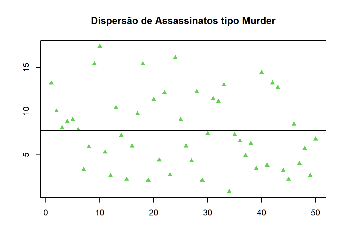 e) verifique se há correlação entre os diferentes tipos de crime.
corrplot(cor(data),method = "circle", type="upper", diag=FALSE,addCoef.col="black",tl.col="black") f) - Verifique se há correlação entre os crimes e a proporção de população urbana.
#Calcular o coeficiente de correlação de Pearson entre duas variaveis
cor ( data, data$UrbanPop, method = "pearson")
## [,1]
## Murder 0.06957262
## Assault 0.25887170
## UrbanPop 1.00000000
## Rape 0.41134124Referencia: ANÁLISE Multivariada - Trabalho 01. Disponível em: https://rpubs.com/viniciusrogerio/usarrests. Acesso em: 30 out. 2022.
install.packages("readr") ## Error in install.packages : Updating loaded packagesimdb <- readr::read_rds("dados/imdb.rds")
imdb## # A tibble: 11,340 × 20
## id_filme titulo ano data_lan…¹ generos duracao pais idioma orcam…² receita recei…³ nota_…⁴ num_a…⁵ direcao roteiro produ…⁶ elenco descr…⁷ num_c…⁸ num_c…⁹
## <chr> <chr> <dbl> <chr> <chr> <dbl> <chr> <chr> <dbl> <dbl> <dbl> <dbl> <dbl> <chr> <chr> <chr> <chr> <chr> <dbl> <dbl>
## 1 tt0092699 Broadcast News 1987 1988-04-01 Comedy… 133 USA Engli… 2 e7 6.73e7 5.12e7 7.2 26257 James … James … Amerce… Willi… Take t… 142 62
## 2 tt0037931 Murder, He Says 1945 1945-06-23 Comedy… 91 USA Engli… NA NA NA 7.1 1639 George… Lou Br… Paramo… Fred … A poll… 35 10
## 3 tt0183505 Me, Myself & Irene 2000 2000-09-08 Comedy 116 USA Engli… 5.1e7 1.49e8 9.06e7 6.6 219069 Bobby … Peter … Twenti… Jim C… A nice… 502 161
## 4 tt0033945 Never Give a Sucker an Even Break 1941 1947-05-02 Comedy… 71 USA Engli… NA NA NA 7.2 2108 Edward… John T… Univer… W.C. … A film… 35 18
## 5 tt0372122 Adam & Steve 2005 2007-05-17 Comedy… 99 USA Engli… NA 3.09e5 3.09e5 5.9 2953 Craig … Craig … Funny … Malco… Follow… 48 15
## 6 tt3703836 Henry Gamble's Birthday Party 2015 2016-01-08 Drama 87 USA Engli… NA NA NA 6.1 2364 Stephe… Stephe… Chicag… Cole … Preach… 26 14
## 7 tt0093640 No Way Out 1987 1987-12-11 Action… 114 USA Engli… 1.5e7 3.55e7 3.55e7 7.1 34513 Roger … Kennet… Orion … Kevin… A cove… 125 72
## 8 tt0494652 Welcome Home, Roscoe Jenkins 2008 2008-02-08 Comedy… 104 USA Engli… 3.5e7 4.37e7 4.24e7 5.5 13315 Malcol… Malcol… Univer… Marti… Dr. RJ… 45 74
## 9 tt0094006 Some Kind of Wonderful 1987 1988-01-13 Drama,… 95 USA Engli… NA 1.86e7 1.86e7 7.1 27065 Howard… John H… Hughes… Eric … When K… 145 55
## 10 tt1142798 The Family That Preys 2008 2008-09-12 Drama 111 USA Engli… NA 3.71e7 3.71e7 5.7 6703 Tyler … Tyler … Louisi… Alfre… Two fa… 52 29
## # … with 11,330 more rows, and abbreviated variable names ¹data_lancamento, ²orcamento, ³receita_eua, ⁴nota_imdb, ⁵num_avaliacoes, ⁶producao, ⁷descricao, ⁸num_criticas_publico,
## # ⁹num_criticas_criticaa). Crie um gráfico de dispersão da nota do imdb pelo orçamento.
plot(imdb$orcamento,xlab="", ylab = "", col = 3, pch = 17, lower.panel=NULL,main="Dispersão de Orçamento")
2.1 Laboratorio – 03
2.1.1 Conjunto de dados inibina
- Faça uma breve análise descritiva dos dados Carregar o conjunto de dados inibina
getwd()## [1] "C:/Users/Administrador/Documents/Biblioteca/Codigo/Rstudio/BIG019"inibina <- read_excel("dados/inibina.xls")
inibina## # A tibble: 32 × 4
## ident resposta inibpre inibpos
## <dbl> <chr> <dbl> <dbl>
## 1 1 positiva 54.0 65.9
## 2 2 positiva 159. 281.
## 3 3 positiva 98.3 305.
## 4 4 positiva 85.3 434.
## 5 5 positiva 128. 229.
## 6 6 positiva 144. 354.
## 7 7 positiva 111. 254.
## 8 8 positiva 47.5 199.
## 9 9 positiva 123. 328.
## 10 10 positiva 166. 339.
## # … with 22 more rowsnrow(inibina)## [1] 32sum()## [1] 0inibina$difinib = inibina$inibpos - inibina$inibpre
#agrupar as respostas e contador a qtde
inibina$resposta = as.factor(inibina$resposta)
plot(inibina$difinib ~ inibina$resposta, ylim = c(0,400))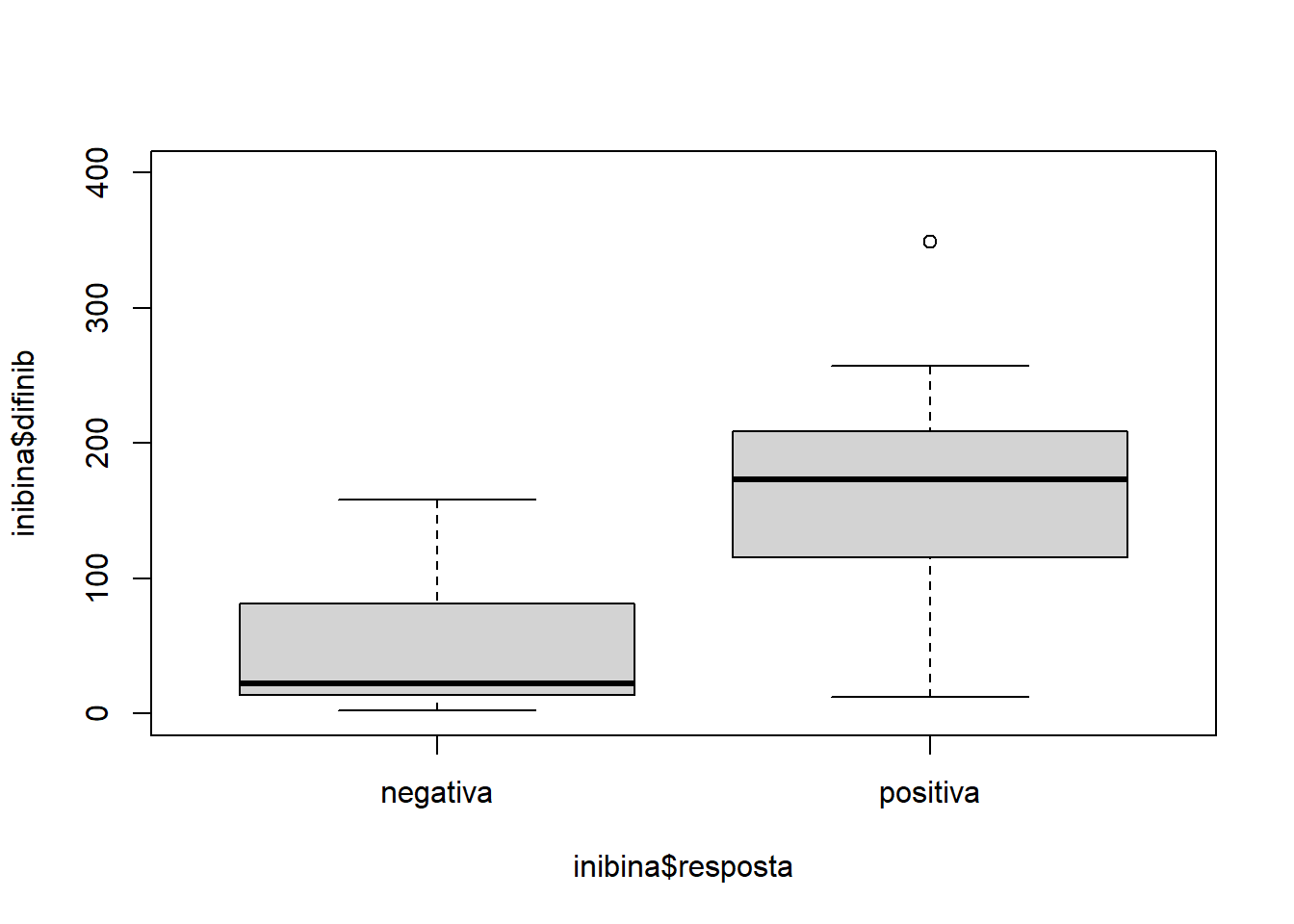
# Hmisc::describe(inibina)

summary(inibina)
## ident resposta inibpre inibpos difinib
## Min. : 1.00 negativa:13 Min. : 3.02 Min. : 6.03 Min. : 2.48
## 1st Qu.: 8.75 positiva:19 1st Qu.: 52.40 1st Qu.: 120.97 1st Qu.: 24.22
## Median :16.50 Median :109.44 Median : 228.89 Median :121.18
## Mean :16.50 Mean :100.53 Mean : 240.80 Mean :140.27
## 3rd Qu.:24.25 3rd Qu.:148.93 3rd Qu.: 330.77 3rd Qu.:183.77
## Max. :32.00 Max. :186.38 Max. :1055.19 Max. :868.81sd( inibina$difinib )## [1] 159.2217modLogist01 = glm( resposta ~ difinib, family = binomial, data = inibina )
summary( modLogist01 )##
## Call:
## glm(formula = resposta ~ difinib, family = binomial, data = inibina)
##
## Deviance Residuals:
## Min 1Q Median 3Q Max
## -1.9770 -0.5594 0.1890 0.5589 2.0631
##
## Coefficients:
## Estimate Std. Error z value Pr(>|z|)
## (Intercept) -2.310455 0.947438 -2.439 0.01474 *
## difinib 0.025965 0.008561 3.033 0.00242 **
## ---
## Signif. codes: 0 '***' 0.001 '**' 0.01 '*' 0.05 '.' 0.1 ' ' 1
##
## (Dispersion parameter for binomial family taken to be 1)
##
## Null deviance: 43.230 on 31 degrees of freedom
## Residual deviance: 24.758 on 30 degrees of freedom
## AIC: 28.758
##
## Number of Fisher Scoring iterations: 6#c. Ajuste um modelo de regressão logística aos dados. Qual é a acurácia do modelo em fazer classificação?
predito = predict.glm( modLogist01, type = "response")
classPred = ifelse(predito>0.5,"positiva", "negativa")
classPred = as.factor(classPred)
confusionMatrix(classPred, inibina$resposta, positive = "positiva" )
## Confusion Matrix and Statistics
##
## Reference
## Prediction negativa positiva
## negativa 10 2
## positiva 3 17
##
## Accuracy : 0.8438
## 95% CI : (0.6721, 0.9472)
## No Information Rate : 0.5938
## P-Value [Acc > NIR] : 0.002273
##
## Kappa : 0.6721
##
## Mcnemar's Test P-Value : 1.000000
##
## Sensitivity : 0.8947
## Specificity : 0.7692
## Pos Pred Value : 0.8500
## Neg Pred Value : 0.8333
## Prevalence : 0.5938
## Detection Rate : 0.5312
## Detection Prevalence : 0.6250
## Balanced Accuracy : 0.8320
##
## 'Positive' Class : positiva
## #d.Use o classificador linear de Fisher para classificar a variável resposta de acordo com a variável preditora.
modFisher01 = lda( resposta ~ difinib, data = inibina, prior = c(0.5 , 0.5))
predito = predict(modFisher01)
confusionMatrix(classPred, inibina$resposta, positive = "positiva")
## Confusion Matrix and Statistics
##
## Reference
## Prediction negativa positiva
## negativa 10 2
## positiva 3 17
##
## Accuracy : 0.8438
## 95% CI : (0.6721, 0.9472)
## No Information Rate : 0.5938
## P-Value [Acc > NIR] : 0.002273
##
## Kappa : 0.6721
##
## Mcnemar's Test P-Value : 1.000000
##
## Sensitivity : 0.8947
## Specificity : 0.7692
## Pos Pred Value : 0.8500
## Neg Pred Value : 0.8333
## Prevalence : 0.5938
## Detection Rate : 0.5312
## Detection Prevalence : 0.6250
## Balanced Accuracy : 0.8320
##
## 'Positive' Class : positiva
## Qual é a acurácia do classificador? 0.8438
#e. Use o classificador linear de Bayes para classificar a variável resposta de acordo com as variáveis explicativas. Utilize priori 0,65 e 0,35 para resposta negativa e positiva, respectivamente.
#inibina$resposta
modBayes01 = lda(resposta ~ difinib, data = inibina, prior = c(0.65, 0.35))
predito = predict(modBayes01)
classPred = predito$class
# table(classPred)
confusionMatrix(classPred, inibina$resposta, positive = "positiva")
## Confusion Matrix and Statistics
##
## Reference
## Prediction negativa positiva
## negativa 13 13
## positiva 0 6
##
## Accuracy : 0.5938
## 95% CI : (0.4064, 0.763)
## No Information Rate : 0.5938
## P-Value [Acc > NIR] : 0.5755484
##
## Kappa : 0.2727
##
## Mcnemar's Test P-Value : 0.0008741
##
## Sensitivity : 0.3158
## Specificity : 1.0000
## Pos Pred Value : 1.0000
## Neg Pred Value : 0.5000
## Prevalence : 0.5938
## Detection Rate : 0.1875
## Detection Prevalence : 0.1875
## Balanced Accuracy : 0.6579
##
## 'Positive' Class : positiva
## Qual é a acurácia do classificador? 0.5938
#f. Use o classificador knn para classificar a variável resposta de acordo com as variáveis preditoras. Utilize k = 1, 3, 5.
modKnn1_01 = knn3(resposta ~ difinib, data = inibina, k = 1)
predito = predict(modKnn1_01, inibina, type = "class")
confusionMatrix(predito, inibina$resposta, positive = "positiva")
## Confusion Matrix and Statistics
##
## Reference
## Prediction negativa positiva
## negativa 13 0
## positiva 0 19
##
## Accuracy : 1
## 95% CI : (0.8911, 1)
## No Information Rate : 0.5938
## P-Value [Acc > NIR] : 5.693e-08
##
## Kappa : 1
##
## Mcnemar's Test P-Value : NA
##
## Sensitivity : 1.0000
## Specificity : 1.0000
## Pos Pred Value : 1.0000
## Neg Pred Value : 1.0000
## Prevalence : 0.5938
## Detection Rate : 0.5938
## Detection Prevalence : 0.5938
## Balanced Accuracy : 1.0000
##
## 'Positive' Class : positiva
## modKnn3_01 = knn3(resposta ~ difinib, data = inibina, k = 3)
predito = predict(modKnn3_01, inibina, type = "class")
confusionMatrix(predito, inibina$resposta, positive = "positiva")## Confusion Matrix and Statistics
##
## Reference
## Prediction negativa positiva
## negativa 11 2
## positiva 2 17
##
## Accuracy : 0.875
## 95% CI : (0.7101, 0.9649)
## No Information Rate : 0.5938
## P-Value [Acc > NIR] : 0.0005536
##
## Kappa : 0.7409
##
## Mcnemar's Test P-Value : 1.0000000
##
## Sensitivity : 0.8947
## Specificity : 0.8462
## Pos Pred Value : 0.8947
## Neg Pred Value : 0.8462
## Prevalence : 0.5938
## Detection Rate : 0.5312
## Detection Prevalence : 0.5938
## Balanced Accuracy : 0.8704
##
## 'Positive' Class : positiva
## modKnn5_01 = knn3(resposta ~ difinib, data = inibina, k = 5)
predito = predict(modKnn5_01, inibina, type = "class")
confusionMatrix(predito, inibina$resposta, positive = "positiva")## Confusion Matrix and Statistics
##
## Reference
## Prediction negativa positiva
## negativa 9 1
## positiva 4 18
##
## Accuracy : 0.8438
## 95% CI : (0.6721, 0.9472)
## No Information Rate : 0.5938
## P-Value [Acc > NIR] : 0.002273
##
## Kappa : 0.6639
##
## Mcnemar's Test P-Value : 0.371093
##
## Sensitivity : 0.9474
## Specificity : 0.6923
## Pos Pred Value : 0.8182
## Neg Pred Value : 0.9000
## Prevalence : 0.5938
## Detection Rate : 0.5625
## Detection Prevalence : 0.6875
## Balanced Accuracy : 0.8198
##
## 'Positive' Class : positiva
## #g. Use naive Bayes para para classificar a variável resposta de acordo com as variáveis preditoras.
library(e1071)
modNaiveBayes01 = naiveBayes(resposta ~ difinib, data = inibina)
predito = predict(modNaiveBayes01, inibina)
confusionMatrix(predito, inibina$resposta, positive = "positiva")
## Confusion Matrix and Statistics
##
## Reference
## Prediction negativa positiva
## negativa 11 5
## positiva 2 14
##
## Accuracy : 0.7812
## 95% CI : (0.6003, 0.9072)
## No Information Rate : 0.5938
## P-Value [Acc > NIR] : 0.02102
##
## Kappa : 0.5625
##
## Mcnemar's Test P-Value : 0.44969
##
## Sensitivity : 0.7368
## Specificity : 0.8462
## Pos Pred Value : 0.8750
## Neg Pred Value : 0.6875
## Prevalence : 0.5938
## Detection Rate : 0.4375
## Detection Prevalence : 0.5000
## Balanced Accuracy : 0.7915
##
## 'Positive' Class : positiva
## #h. Use uma arvore de decisão para classificar a variável resposta de acordo com as variáveis preditoras
install.packages('rpart')## Warning in install.packages :
## package 'rpart' is in use and will not be installedlibrary(rpart)
library(rpart.plot)
modArvDec01 = rpart(resposta ~ difinib, data = inibina)
prp(modArvDec01, faclen=0, #use full names for factor labels
extra=1, #display number of observations for each terminal node
roundint=F, #don't round to integers in output
digits=5)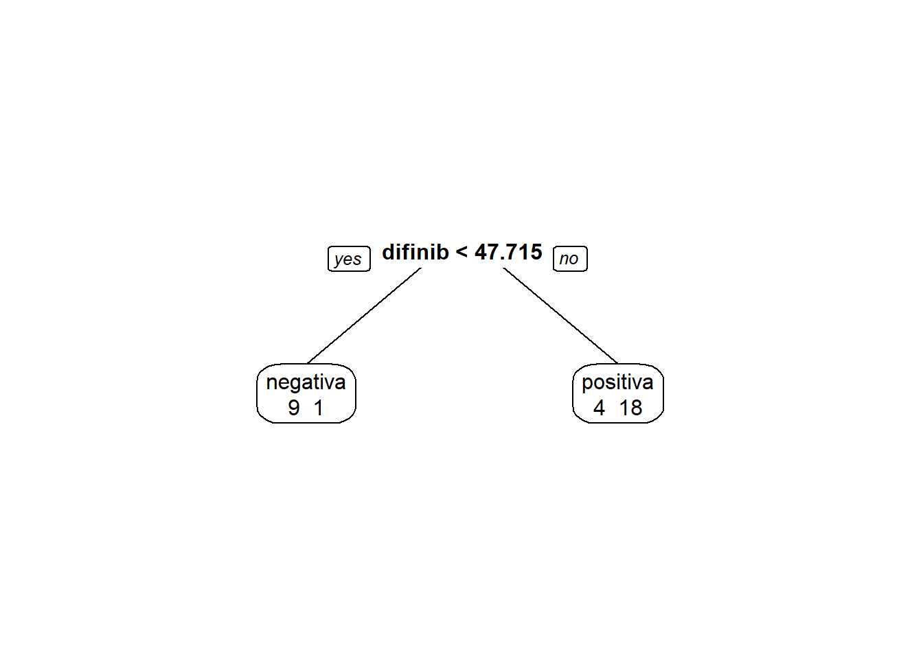
predito = predict(modArvDec01, type = "class")
confusionMatrix(predito, inibina$resposta, positive = "positiva")
## Confusion Matrix and Statistics
##
## Reference
## Prediction negativa positiva
## negativa 9 1
## positiva 4 18
##
## Accuracy : 0.8438
## 95% CI : (0.6721, 0.9472)
## No Information Rate : 0.5938
## P-Value [Acc > NIR] : 0.002273
##
## Kappa : 0.6639
##
## Mcnemar's Test P-Value : 0.371093
##
## Sensitivity : 0.9474
## Specificity : 0.6923
## Pos Pred Value : 0.8182
## Neg Pred Value : 0.9000
## Prevalence : 0.5938
## Detection Rate : 0.5625
## Detection Prevalence : 0.6875
## Balanced Accuracy : 0.8198
##
## 'Positive' Class : positiva
## #i. Use SVM para fazer para classificar a variável resposta de acordo com as variáveis preditoras.
x = 1:32
plot(inibina$difinib ~x, col = inibina$resposta)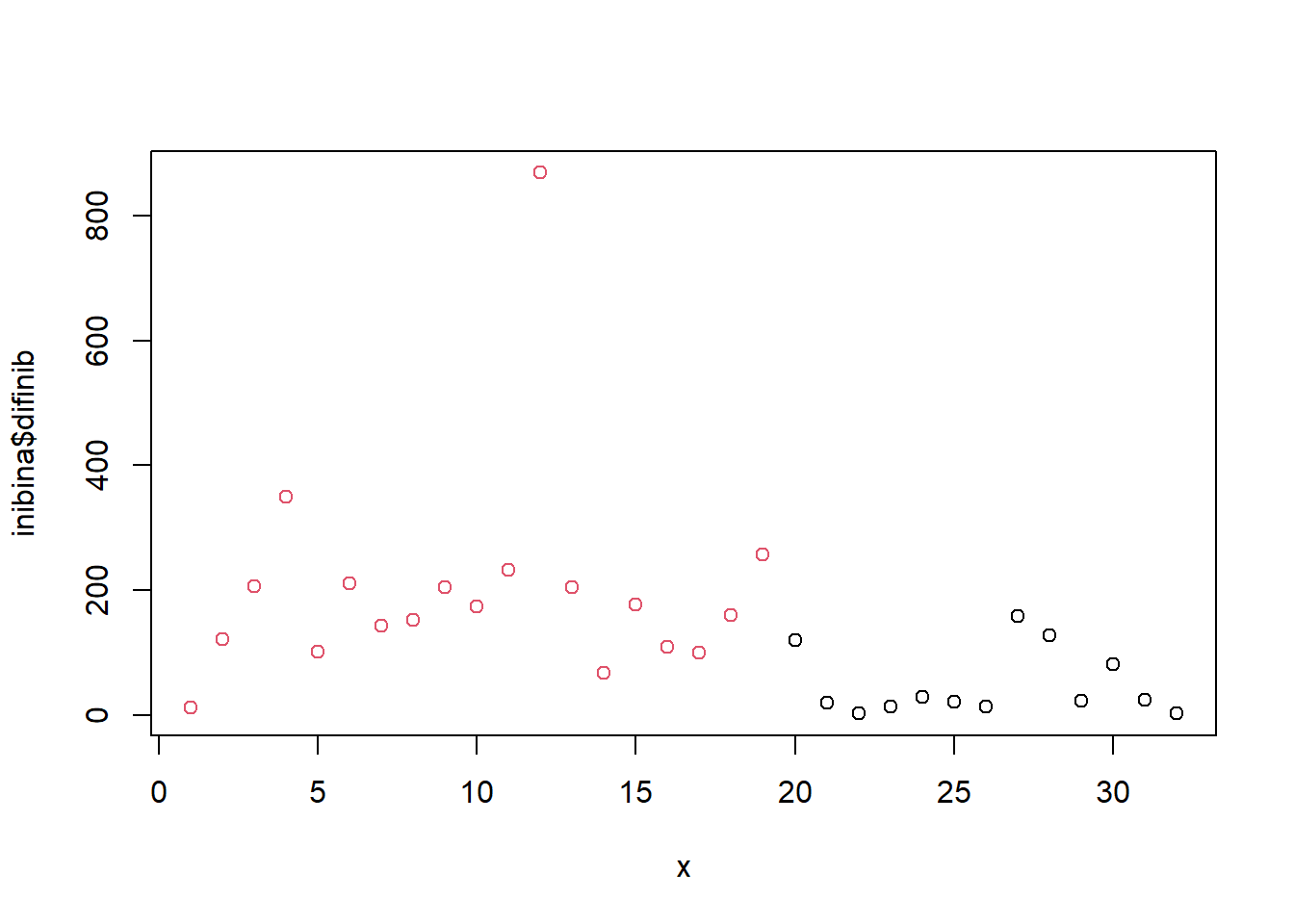
modSVM01 = svm(resposta ~ difinib, data = inibina, kernel = "linear")

predito = predict(modSVM01, type = "class")
confusionMatrix(predito, inibina$resposta, positive = "positiva")
## Confusion Matrix and Statistics
##
## Reference
## Prediction negativa positiva
## negativa 10 2
## positiva 3 17
##
## Accuracy : 0.8438
## 95% CI : (0.6721, 0.9472)
## No Information Rate : 0.5938
## P-Value [Acc > NIR] : 0.002273
##
## Kappa : 0.6721
##
## Mcnemar's Test P-Value : 1.000000
##
## Sensitivity : 0.8947
## Specificity : 0.7692
## Pos Pred Value : 0.8500
## Neg Pred Value : 0.8333
## Prevalence : 0.5938
## Detection Rate : 0.5312
## Detection Prevalence : 0.6250
## Balanced Accuracy : 0.8320
##
## 'Positive' Class : positiva
## #j. Use uma rede neural para classificar a variável resposta de acordo com as variáveis preditoras.
#install.packages("neuralnet")
#library(neuralnet)
library("neuralnet")

modRedNeural01 = neuralnet(resposta ~ difinib, data = inibina, hidden = c(2,4,3))
plot(modRedNeural01)

ypred = neuralnet::compute(modRedNeural01, inibina)
yhat = ypred$net.resultround(yhat)## [,1] [,2]
## [1,] 1 0
## [2,] 0 1
## [3,] 0 1
## [4,] 0 1
## [5,] 0 1
## [6,] 0 1
## [7,] 0 1
## [8,] 0 1
## [9,] 0 1
## [10,] 0 1
## [11,] 0 1
## [12,] 0 1
## [13,] 0 1
## [14,] 0 1
## [15,] 0 1
## [16,] 0 1
## [17,] 0 1
## [18,] 0 1
## [19,] 0 1
## [20,] 0 1
## [21,] 1 0
## [22,] 1 0
## [23,] 1 0
## [24,] 1 0
## [25,] 1 0
## [26,] 1 0
## [27,] 0 1
## [28,] 0 1
## [29,] 1 0
## [30,] 0 1
## [31,] 1 0
## [32,] 1 0yhat=data.frame("yhat"=ifelse(max.col(yhat[ ,1:2])==1, "negativa", "positiva"))
cm = confusionMatrix(inibina$resposta, as.factor(yhat$yhat))
print(cm)## Confusion Matrix and Statistics
##
## Reference
## Prediction negativa positiva
## negativa 9 4
## positiva 1 18
##
## Accuracy : 0.8438
## 95% CI : (0.6721, 0.9472)
## No Information Rate : 0.6875
## P-Value [Acc > NIR] : 0.03739
##
## Kappa : 0.6639
##
## Mcnemar's Test P-Value : 0.37109
##
## Sensitivity : 0.9000
## Specificity : 0.8182
## Pos Pred Value : 0.6923
## Neg Pred Value : 0.9474
## Prevalence : 0.3125
## Detection Rate : 0.2812
## Detection Prevalence : 0.4062
## Balanced Accuracy : 0.8591
##
## 'Positive' Class : negativa
## #k. Refaça os itens c à j usando o método de validação cruzada leave-one-out. Dica: use a função train do pacote caret.
library(caret)
library(tibble)

trControl <- trainControl(method = "LOOCV")

fit <- train(resposta ~ difinib, method = "glm", data = inibina,
             trControl = trControl, metric = "Accuracy")
fit <- train(resposta ~ difinib, method = "lda", data = inibina, prior = c(0.5, 0.5),
             trControl = trControl, metric = "Accuracy")
fit <- train(resposta ~ difinib, method = "lda", data = inibina, prior = c(0.65, 0.35),
             trControl = trControl, metric = "Accuracy")
fit <- train(resposta ~ difinib, method = "knn", data = inibina,
             tuneGrid = expand.grid(k = 1:5),
             trControl = trControl, metric = "Accuracy")

totalAcerto = 0
for (i in 1:nrow(inibina)){
    treino = inibina[-i,]
    teste = inibina[i,]
    modelo = svm(resposta ~ difinib, data = treino)
    predito = predict(modelo, newdata = teste,  type = "class")
    if(predito == teste$resposta[1])  totalAcerto = totalAcerto+1
}

iris = tibble(iris)
irisS = iris[,1:4]

d <- dist(irisS, method = "maximum")
grup = hclust(d, method = "ward.D")
plot(grup, cex = 0.6)

groups <- cutree(grup, k=3)
table(groups, iris$Species)
##
## groups setosa versicolor virginica
## 1 50 0 0
## 2 0 50 15
## 3 0 0 35rect.hclust(grup, k=3, border="red")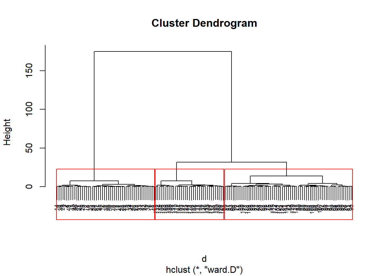
install.packages("factoextra")## Warning in install.packages :
## package 'factoextra' is in use and will not be installedlibrary(factoextra)
library(ggpubr)
km1 = kmeans(irisS, 4)
p1 = fviz_cluster(km1, data=irisS,
palette = c("#2E9FDF", "#FC4E07", "#E7B800", "#E7B700"),
star.plot=FALSE,
# repel=TRUE,
ggtheme=theme_bw())
p1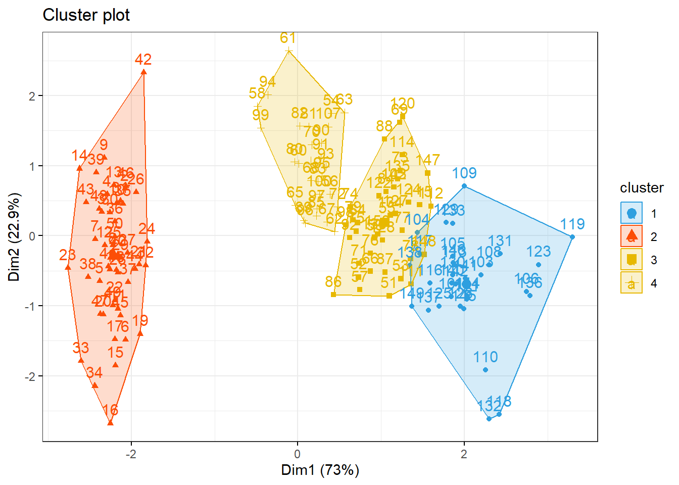
groups = km1$cluster
table(groups, iris$Species)
##
## groups setosa versicolor virginica
## 1 0 0 32
## 2 50 0 0
## 3 0 23 17
## 4 0 27 1#Qual classificador você escolheria? Resp.: Muito modelos apresentaram uma acuracia abaixo de 0,90. Apenas o modelo KNN chegou a uma acucaria de 1. Desta forma, seleciono o modelo KNN.
#——————————————————————————–
2.1.2 Conjunto de dados Hospital Universitário
#a. Qual é a variável resposta e quais são as explicativas? Faça uma breve análise descritiva dos dados.
Variavel resposta: medidas obtidas ultrassonograficamente Explicativas: Distâncias cápsula-côndilo (em mm) com boca aberta ou fechada Disco correspondente foi classificado como deslocado (1) ou não (0)
#b. Como você modelaria esse conjunto de dados?
Importando os dados
tabdisc <- read_excel("dados/disco.xls")
tabdisc
## # A tibble: 104 × 3
## deslocamento distanciaA distanciaF
## <dbl> <dbl> <dbl>
## 1 0 2.2 1.4
## 2 0 2.4 1.2
## 3 0 2.6 2
## 4 1 3.5 1.8
## 5 0 1.3 1
## 6 1 2.8 1.1
## 7 0 1.5 1.2
## 8 0 2.6 1.1
## 9 0 1.2 0.6
## 10 0 1.7 1.5
## # … with 94 more rowsn = length(tabdisc$deslocamento)
res <- paste("Tamanho da amostra: ", n)
print(res )## [1] "Tamanho da amostra: 104"#Inspecionado a estrutura de dados #Lista tipo de dados do DataFrame
str(tabdisc)## tibble [104 × 3] (S3: tbl_df/tbl/data.frame)
## $ deslocamento: num [1:104] 0 0 0 1 0 1 0 0 0 0 ...
## $ distanciaA : num [1:104] 2.2 2.4 2.6 3.5 1.3 2.8 1.5 2.6 1.2 1.7 ...
## $ distanciaF : num [1:104] 1.4 1.2 2 1.8 1 1.1 1.2 1.1 0.6 1.5 ...#Lista os rotulo das colunas
names(tabdisc)## [1] "deslocamento" "distanciaA" "distanciaF"#Tamanho do DataSet Linhas e Colunas
dim(tabdisc)## [1] 104 3#Agrupando as respostas e somando a distanciaA e distanciaB
tabdisc$soma = tabdisc$distanciaA + tabdisc$distanciaF
tabdisc$descolamento = as.factor(tabdisc$deslocamento)
plot(tabdisc$soma ~ tabdisc$descolamento, ylim = c(0,10))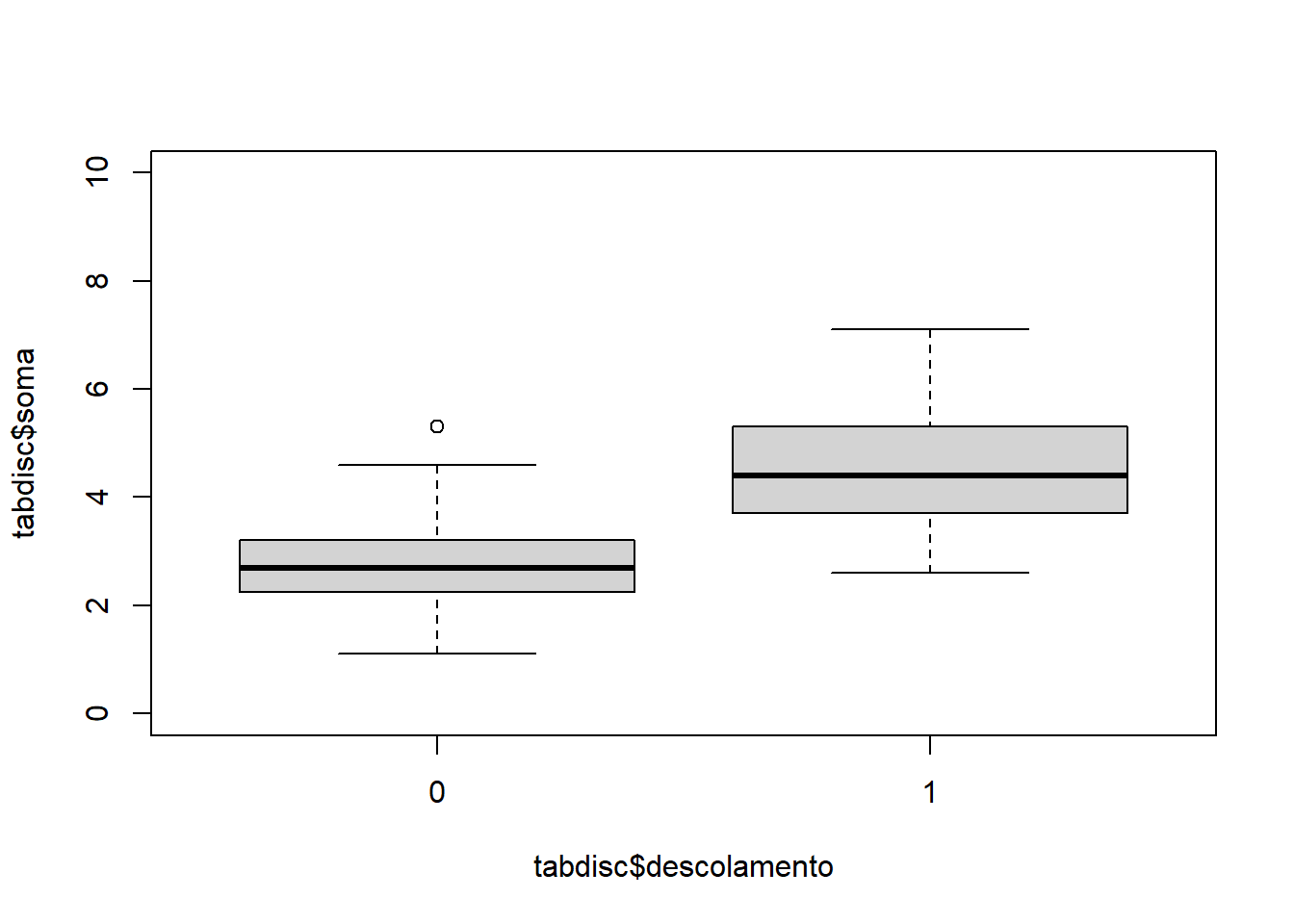 #Gráfico de dispersão da Distancia Aberto e Fechada
#plot(tabdisc$distanciaA ~ tabdisc$distanciaF , col=tabdisc$deslocamento, ylim = c(0,100000) )
plot(tabdisc$distanciaA, col=tabdisc$distanciaF)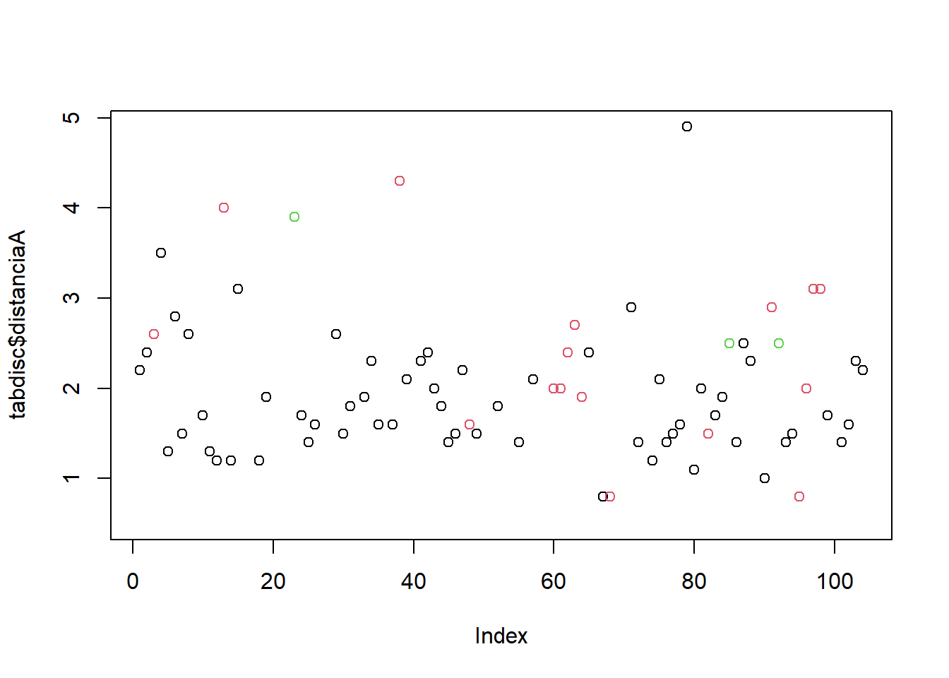
#Sumarizando os dados importados
summary(tabdisc)## deslocamento distanciaA distanciaF soma descolamento
## Min. :0.0000 Min. :0.500 Min. :0.400 Min. :1.100 0:75
## 1st Qu.:0.0000 1st Qu.:1.400 1st Qu.:1.000 1st Qu.:2.500 1:29
## Median :0.0000 Median :1.700 Median :1.200 Median :2.900
## Mean :0.2788 Mean :1.907 Mean :1.362 Mean :3.268
## 3rd Qu.:1.0000 3rd Qu.:2.300 3rd Qu.:1.600 3rd Qu.:3.700
## Max. :1.0000 Max. :4.900 Max. :3.300 Max. :7.100#c. Separe o conjunto de dados em conjunto de treinamento (70% dos dados) e conjunto de teste (30%).
tabdisc$descolamento## [1] 0 0 0 1 0 1 0 0 0 0 0 0 1 0 1 1 0 0 0 0 1 0 1 0 0 0 0 0 1 0 0 0 0 0 0 0 0 1 0 0 0 0 0 0 0 0 0 0 0 0 0 0 0 0 0 0 0 0 0 0 0 0 1 1 1 1 0 1 0 0 1 0 1 0 1 1 0 0 1 0 1 0 0 0 1 0 1 1 0 0 1
## [92] 1 0 0 0 0 1 1 0 0 0 0 1 1
## Levels: 0 1modBayes01 = lda(descolamento ~ soma, data = tabdisc, prior = c(0.70, 0.30))
predito = predict(modBayes01)
classPred = predito$class
confusionMatrix(classPred, tabdisc$descolamento)## Confusion Matrix and Statistics
##
## Reference
## Prediction 0 1
## 0 70 13
## 1 5 16
##
## Accuracy : 0.8269
## 95% CI : (0.7403, 0.8941)
## No Information Rate : 0.7212
## P-Value [Acc > NIR] : 0.00857
##
## Kappa : 0.5299
##
## Mcnemar's Test P-Value : 0.09896
##
## Sensitivity : 0.9333
## Specificity : 0.5517
## Pos Pred Value : 0.8434
## Neg Pred Value : 0.7619
## Prevalence : 0.7212
## Detection Rate : 0.6731
## Detection Prevalence : 0.7981
## Balanced Accuracy : 0.7425
##
## 'Positive' Class : 0
## #d. Ajuste um modelo de regressão logística conjunto de treinamento. Qual é a acurácia do modelo no conjunto de teste? Modelo 1
modBayes01 = lda(descolamento ~ soma, data = tabdisc, prior = c(0.65, 0.35))
predito = predict(modBayes01)
classPred = predito$class
confusionMatrix(classPred, tabdisc$descolamento)
## Confusion Matrix and Statistics
##
## Reference
## Prediction 0 1
## 0 70 12
## 1 5 17
##
## Accuracy : 0.8365
## 95% CI : (0.7512, 0.9018)
## No Information Rate : 0.7212
## P-Value [Acc > NIR] : 0.004313
##
## Kappa : 0.5611
##
## Mcnemar's Test P-Value : 0.145610
##
## Sensitivity : 0.9333
## Specificity : 0.5862
## Pos Pred Value : 0.8537
## Neg Pred Value : 0.7727
## Prevalence : 0.7212
## Detection Rate : 0.6731
## Detection Prevalence : 0.7885
## Balanced Accuracy : 0.7598
##
## 'Positive' Class : 0
## Modelo 2
modBayes01 = lda(descolamento ~ soma, data = tabdisc, prior = c(0.60, 0.40))
predito = predict(modBayes01)
classPred = predito$class
confusionMatrix(classPred, tabdisc$descolamento)
## Confusion Matrix and Statistics
##
## Reference
## Prediction 0 1
## 0 70 9
## 1 5 20
##
## Accuracy : 0.8654
## 95% CI : (0.7845, 0.9244)
## No Information Rate : 0.7212
## P-Value [Acc > NIR] : 0.0003676
##
## Kappa : 0.6505
##
## Mcnemar's Test P-Value : 0.4226781
##
## Sensitivity : 0.9333
## Specificity : 0.6897
## Pos Pred Value : 0.8861
## Neg Pred Value : 0.8000
## Prevalence : 0.7212
## Detection Rate : 0.6731
## Detection Prevalence : 0.7596
## Balanced Accuracy : 0.8115
##
## 'Positive' Class : 0
## Modelo 3
modBayes01 = lda(descolamento ~ soma, data = tabdisc, prior = c(0.80, 0.20))
predito = predict(modBayes01)
classPred = predito$class
confusionMatrix(classPred, tabdisc$descolamento)
## Confusion Matrix and Statistics
##
## Reference
## Prediction 0 1
## 0 71 13
## 1 4 16
##
## Accuracy : 0.8365
## 95% CI : (0.7512, 0.9018)
## No Information Rate : 0.7212
## P-Value [Acc > NIR] : 0.004313
##
## Kappa : 0.5508
##
## Mcnemar's Test P-Value : 0.052345
##
## Sensitivity : 0.9467
## Specificity : 0.5517
## Pos Pred Value : 0.8452
## Neg Pred Value : 0.8000
## Prevalence : 0.7212
## Detection Rate : 0.6827
## Detection Prevalence : 0.8077
## Balanced Accuracy : 0.7492
##
## 'Positive' Class : 0
## #e. Use o classificador de Fisher para classificar a variável resposta de acordo com a variável preditora. Qual é a acurácia do classificador? Ajuste o modelo no conjunto de treino e faça a predição no conjunto de teste
modFisher01 = lda(descolamento ~ soma, data = tabdisc, prior = c(0.5, 0.5))
predito = predict(modFisher01)
classPred = predito$class
confusionMatrix(classPred, tabdisc$descolamento)
## Confusion Matrix and Statistics
##
## Reference
## Prediction 0 1
## 0 67 6
## 1 8 23
##
## Accuracy : 0.8654
## 95% CI : (0.7845, 0.9244)
## No Information Rate : 0.7212
## P-Value [Acc > NIR] : 0.0003676
##
## Kappa : 0.6722
##
## Mcnemar's Test P-Value : 0.7892680
##
## Sensitivity : 0.8933
## Specificity : 0.7931
## Pos Pred Value : 0.9178
## Neg Pred Value : 0.7419
## Prevalence : 0.7212
## Detection Rate : 0.6442
## Detection Prevalence : 0.7019
## Balanced Accuracy : 0.8432
##
## 'Positive' Class : 0
## #f. Use o classificador de Bayes para classificar a variável resposta de acordo com a variável preditora. Utilize priori 0,65 e 0,35 para 0 e 1, respectivamente. Qual é a acurácia do classificador? Ajuste o modelo no conjunto de treino e faça a predição no conjunto de teste.
modBayes01 = lda(descolamento ~ soma, data = tabdisc, prior = c(0.65, 0.35))
predito = predict(modBayes01)
classPred = predito$class
confusionMatrix(classPred, tabdisc$descolamento)
## Confusion Matrix and Statistics
##
## Reference
## Prediction 0 1
## 0 70 12
## 1 5 17
##
## Accuracy : 0.8365
## 95% CI : (0.7512, 0.9018)
## No Information Rate : 0.7212
## P-Value [Acc > NIR] : 0.004313
##
## Kappa : 0.5611
##
## Mcnemar's Test P-Value : 0.145610
##
## Sensitivity : 0.9333
## Specificity : 0.5862
## Pos Pred Value : 0.8537
## Neg Pred Value : 0.7727
## Prevalence : 0.7212
## Detection Rate : 0.6731
## Detection Prevalence : 0.7885
## Balanced Accuracy : 0.7598
##
## 'Positive' Class : 0
## #g. Use o classificador knn para classificar a variável resposta de acordo com a variável preditora. Utilize k = 1, 3, 5. Ajuste o modelo no conjunto de treino e faça a predição no conjunto de teste.
modKnn1_01 = knn3(descolamento ~ soma, data = tabdisc, k = 1)
predito = predict(modKnn1_01, tabdisc, type = "class")
confusionMatrix(predito,tabdisc$descolamento)
## Confusion Matrix and Statistics
##
## Reference
## Prediction 0 1
## 0 70 10
## 1 5 19
##
## Accuracy : 0.8558
## 95% CI : (0.7733, 0.917)
## No Information Rate : 0.7212
## P-Value [Acc > NIR] : 0.0008967
##
## Kappa : 0.6214
##
## Mcnemar's Test P-Value : 0.3016996
##
## Sensitivity : 0.9333
## Specificity : 0.6552
## Pos Pred Value : 0.8750
## Neg Pred Value : 0.7917
## Prevalence : 0.7212
## Detection Rate : 0.6731
## Detection Prevalence : 0.7692
## Balanced Accuracy : 0.7943
##
## 'Positive' Class : 0
## modKnn3_01 = knn3(descolamento ~ soma, data = tabdisc, k = 3)
predito = predict(modKnn3_01, tabdisc, type = "class")
confusionMatrix(predito,tabdisc$descolamento)## Confusion Matrix and Statistics
##
## Reference
## Prediction 0 1
## 0 71 8
## 1 4 21
##
## Accuracy : 0.8846
## 95% CI : (0.8071, 0.9389)
## No Information Rate : 0.7212
## P-Value [Acc > NIR] : 4.877e-05
##
## Kappa : 0.7004
##
## Mcnemar's Test P-Value : 0.3865
##
## Sensitivity : 0.9467
## Specificity : 0.7241
## Pos Pred Value : 0.8987
## Neg Pred Value : 0.8400
## Prevalence : 0.7212
## Detection Rate : 0.6827
## Detection Prevalence : 0.7596
## Balanced Accuracy : 0.8354
##
## 'Positive' Class : 0
## modKnn5_01 = knn3(descolamento ~ soma, data = tabdisc, k = 5)
predito = predict(modKnn5_01, tabdisc, type = "class")
confusionMatrix(predito, tabdisc$descolamento)## Confusion Matrix and Statistics
##
## Reference
## Prediction 0 1
## 0 70 8
## 1 5 21
##
## Accuracy : 0.875
## 95% CI : (0.7957, 0.9317)
## No Information Rate : 0.7212
## P-Value [Acc > NIR] : 0.0001395
##
## Kappa : 0.679
##
## Mcnemar's Test P-Value : 0.5790997
##
## Sensitivity : 0.9333
## Specificity : 0.7241
## Pos Pred Value : 0.8974
## Neg Pred Value : 0.8077
## Prevalence : 0.7212
## Detection Rate : 0.6731
## Detection Prevalence : 0.7500
## Balanced Accuracy : 0.8287
##
## 'Positive' Class : 0
## #h. Use naive Bayes para classificar a variável resposta de acordo com as variáveis preditoras. Ajuste o modelo no conjunto de treino e faça a predição no conjunto de teste.
library(e1071)
modNaiveBayes01 = naiveBayes(descolamento ~ soma, data = tabdisc)
predito = predict(modNaiveBayes01, tabdisc)
confusionMatrix(predito, tabdisc$descolamento)
## Confusion Matrix and Statistics
##
## Reference
## Prediction 0 1
## 0 70 13
## 1 5 16
##
## Accuracy : 0.8269
## 95% CI : (0.7403, 0.8941)
## No Information Rate : 0.7212
## P-Value [Acc > NIR] : 0.00857
##
## Kappa : 0.5299
##
## Mcnemar's Test P-Value : 0.09896
##
## Sensitivity : 0.9333
## Specificity : 0.5517
## Pos Pred Value : 0.8434
## Neg Pred Value : 0.7619
## Prevalence : 0.7212
## Detection Rate : 0.6731
## Detection Prevalence : 0.7981
## Balanced Accuracy : 0.7425
##
## 'Positive' Class : 0
## #j. Use svm para fazer para classificar a variável resposta de acordo com as variáveis preditoras. Ajuste o modelo no conjunto de treino e faça a predição no conjunto de teste.
plot(tabdisc$deslocamento, col = tabdisc$soma)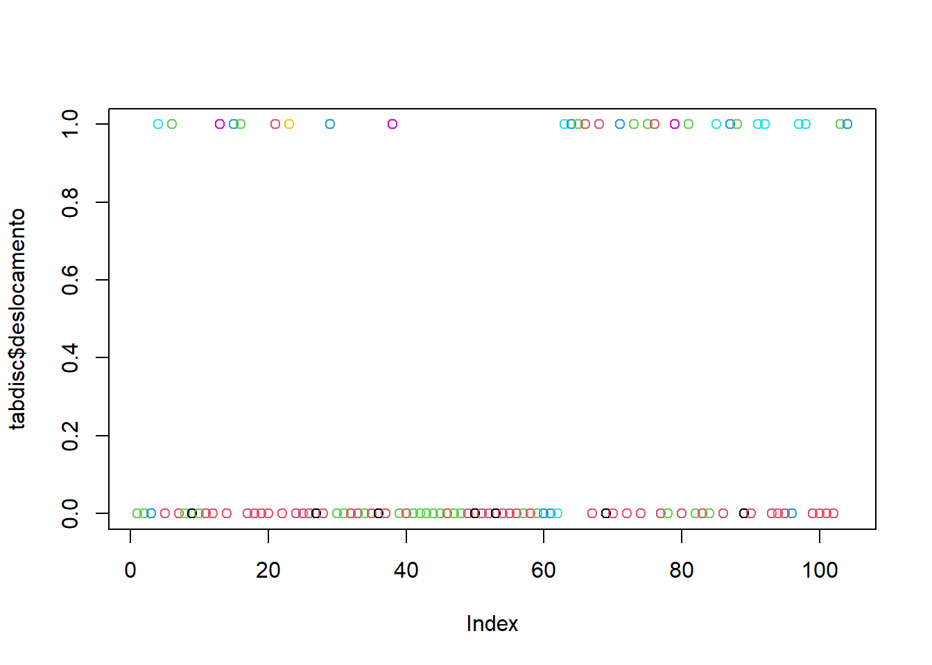
modSVM01 = svm(descolamento ~ soma, data = tabdisc, kernel = "linear")

predito = predict(modSVM01, type = "class")
confusionMatrix(predito, tabdisc$descolamento)
## Confusion Matrix and Statistics
##
## Reference
## Prediction 0 1
## 0 71 13
## 1 4 16
##
## Accuracy : 0.8365
## 95% CI : (0.7512, 0.9018)
## No Information Rate : 0.7212
## P-Value [Acc > NIR] : 0.004313
##
## Kappa : 0.5508
##
## Mcnemar's Test P-Value : 0.052345
##
## Sensitivity : 0.9467
## Specificity : 0.5517
## Pos Pred Value : 0.8452
## Neg Pred Value : 0.8000
## Prevalence : 0.7212
## Detection Rate : 0.6827
## Detection Prevalence : 0.8077
## Balanced Accuracy : 0.7492
##
## 'Positive' Class : 0
## #Use uma rede neural para classificar a variável resposta de acordo com as variáveis preditoras. Ajuste o modelo no conjunto de treino e faça a predição no conjunto de teste.
library(neuralnet)

modRedNeural01 = neuralnet(descolamento ~ soma, data = tabdisc, hidden = c(2,4,3))
plot(modRedNeural01)

ypred = neuralnet::compute(modRedNeural01, tabdisc)
yhat = ypred$net.result

round(yhat)
## [,1] [,2]
## [1,] 1 0
## [2,] 1 0
## [3,] 0 1
## [4,] 0 1
## [5,] 1 0
## [6,] 0 1
## [7,] 1 0
## [8,] 0 0
## [9,] 1 0
## [10,] 1 0
## [11,] 1 0
## [12,] 1 0
## [13,] 0 1
## [14,] 1 0
## [15,] 0 1
## [16,] 1 0
## [17,] 1 0
## [18,] 1 0
## [19,] 1 0
## [20,] 1 0
## [21,] 1 0
## [22,] 1 0
## [23,] 0 1
## [24,] 1 0
## [25,] 1 0
## [26,] 1 0
## [27,] 1 0
## [28,] 1 0
## [29,] 0 1
## [30,] 1 0
## [31,] 1 0
## [32,] 1 0
## [33,] 1 0
## [34,] 1 0
## [35,] 1 0
## [36,] 1 0
## [37,] 1 0
## [38,] 0 1
## [39,] 1 0
## [40,] 1 0
## [41,] 1 0
## [42,] 0 0
## [43,] 1 0
## [44,] 1 0
## [45,] 1 0
## [46,] 1 0
## [47,] 1 0
## [48,] 1 0
## [49,] 1 0
## [50,] 1 0
## [51,] 1 0
## [52,] 1 0
## [53,] 1 0
## [54,] 1 0
## [55,] 1 0
## [56,] 1 0
## [57,] 1 0
## [58,] 1 0
## [59,] 1 0
## [60,] 1 0
## [61,] 1 0
## [62,] 0 1
## [63,] 0 1
## [64,] 0 1
## [65,] 0 0
## [66,] 1 0
## [67,] 1 0
## [68,] 1 0
## [69,] 1 0
## [70,] 1 0
## [71,] 0 1
## [72,] 1 0
## [73,] 0 0
## [74,] 1 0
## [75,] 0 0
## [76,] 1 0
## [77,] 1 0
## [78,] 1 0
## [79,] 0 1
## [80,] 1 0
## [81,] 1 0
## [82,] 0 0
## [83,] 1 0
## [84,] 1 0
## [85,] 0 1
## [86,] 1 0
## [87,] 1 0
## [88,] 0 1
## [89,] 1 0
## [90,] 1 0
## [91,] 0 1
## [92,] 0 1
## [93,] 1 0
## [94,] 1 0
## [95,] 1 0
## [96,] 1 0
## [97,] 0 1
## [98,] 0 1
## [99,] 1 0
## [100,] 1 0
## [101,] 1 0
## [102,] 1 0
## [103,] 0 1
## [104,] 0 1#Qual classificador você escolheria? O modelo que apresentou uma melhor acuracia quando comparado aos demais, o modelo selecionado, foi o KNN com uma acuracia de 0,88
2.1.3 Conjunto de dados do arquivo tipofacial
tabfacial <- read_excel("dados/tipofacial.xls")
tabfacial
## # A tibble: 101 × 13
## paciente sexo grupo idade nsba ns sba altfac proffac eixofac planmand arcomand vert
## <dbl> <chr> <chr> <dbl> <dbl> <dbl> <dbl> <dbl> <dbl> <dbl> <dbl> <dbl> <dbl>
## 1 10 M braq 5.58 132 58 36 1.2 0.8 0.4 0.4 2.5 1.06
## 2 10 M braq 11.4 134 63 42.5 1.2 0.4 1 1 3.6 1.44
## 3 27 F braq 16.2 122. 77.5 48 2.6 0.2 0.3 0.9 3.4 1.48
## 4 39 F braq 4.92 130. 64 34.5 3.1 -1 1.9 1.3 1.6 1.38
## 5 39 F braq 10.9 130. 70 36.5 3.1 0.6 1.2 2.2 2.3 1.88
## 6 39 F braq 12.9 128 68.5 41.5 3.3 -0.6 1.1 1.2 2.1 1.42
## 7 55 F braq 16.8 130 71 42 2.4 0.3 1.1 1.2 3.5 1.7
## 8 76 F braq 16 125 72 46.5 1.9 0.5 1.4 0.6 3.5 1.58
## 9 77 F braq 17.1 130. 70 44 2.1 -0.1 2.2 0.8 0.7 1.14
## 10 133 M braq 14.8 130 80 52 2.8 0.2 0.4 1.1 1.8 1.26
## # … with 91 more rows#a. faça uma breve análise descritiva. Desenhe um gráfico das variáveis altura facial X profundidade facial e marque cada observação de acordo com o tipo facial do indivíduo.
tabfacial$soma = tabfacial$altfac + tabfacial$proffac
tabfacial$grupo = as.factor(tabfacial$grupo)
plot(tabfacial$altfac ~ tabfacial$grupo)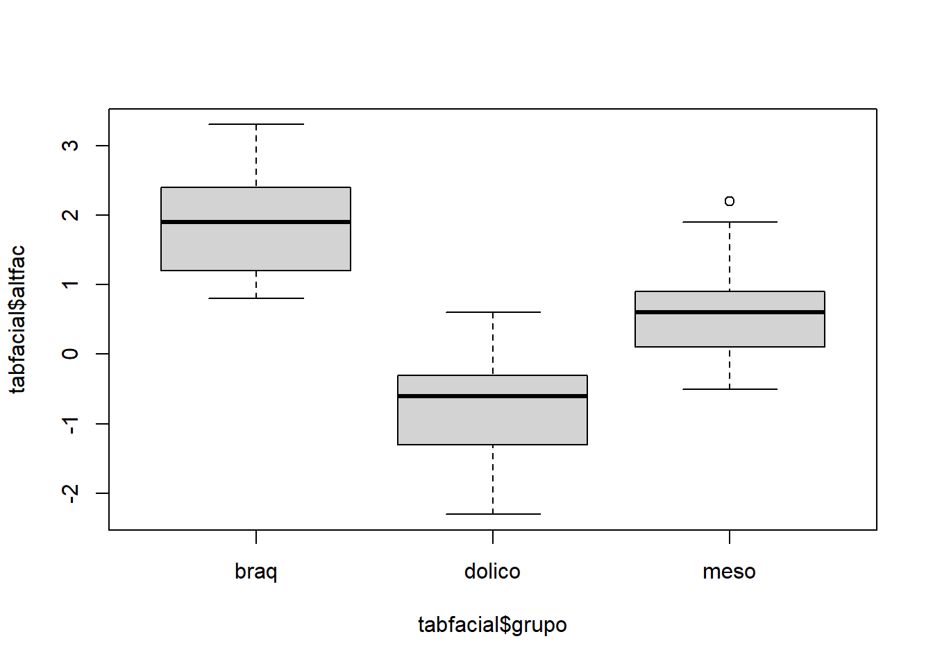
plot(tabfacial$proffac ~ tabfacial$grupo)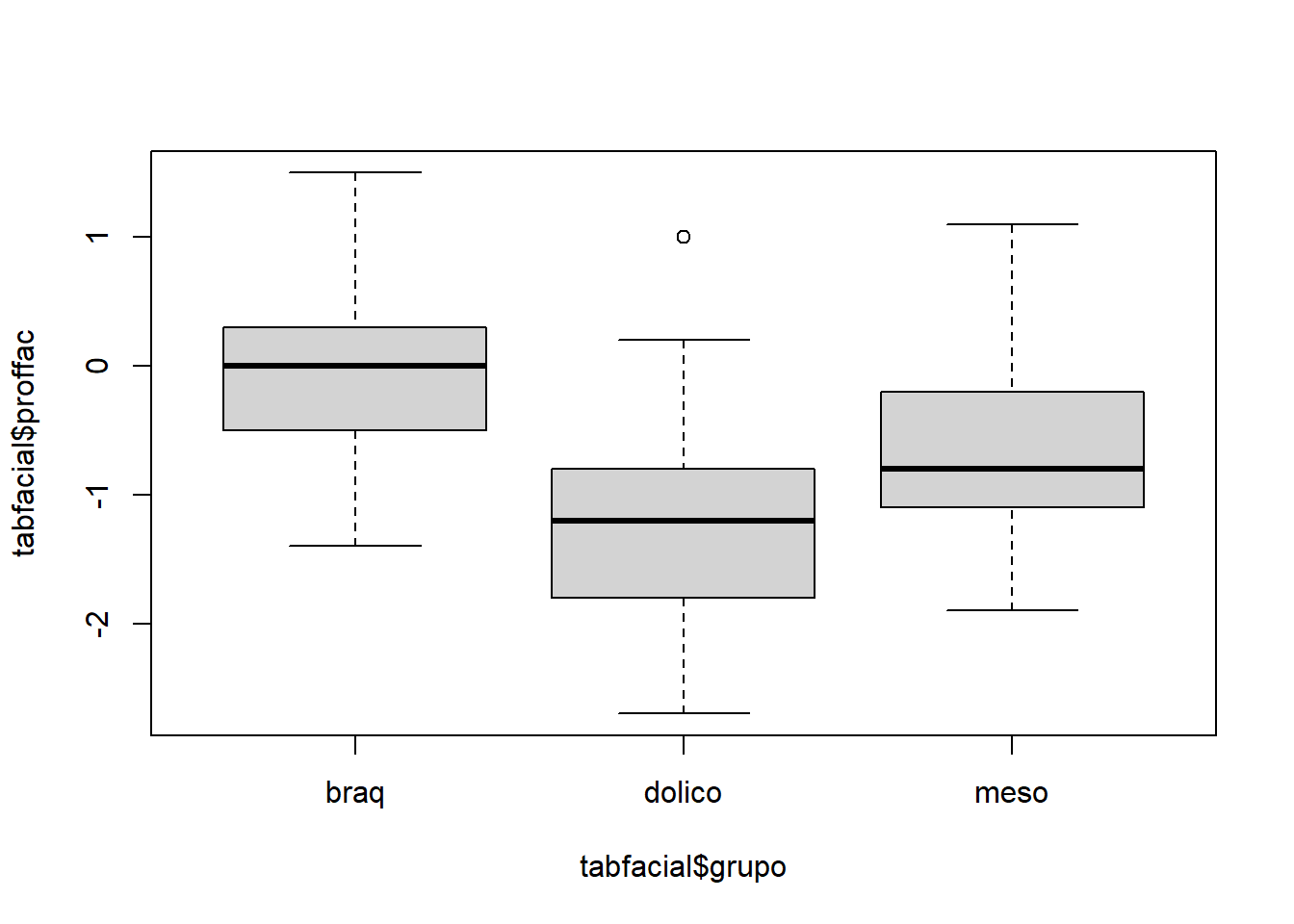
plot(tabfacial$altfac ~ tabfacial$proffac, col=tabfacial$grupo)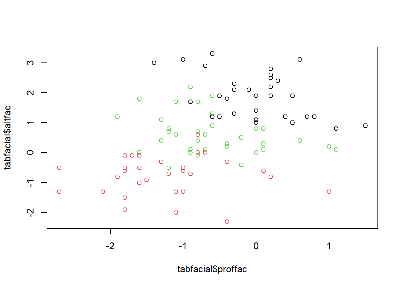
#b. Separe o conjunto de dados em conjunto de treinamento (70% dos dados) e conjunto de teste (30%). Faça isso de 5 formas diferentes. MOdelo 1
modBayes01 = lda(grupo ~ soma, data = tabfacial)
predito = predict(modBayes01)
classPred = predito$class
confusionMatrix(classPred, tabfacial$grupo)
## Confusion Matrix and Statistics
##
## Reference
## Prediction braq dolico meso
## braq 29 0 5
## dolico 0 23 2
## meso 4 8 30
##
## Overall Statistics
##
## Accuracy : 0.8119
## 95% CI : (0.7219, 0.8828)
## No Information Rate : 0.3663
## P-Value [Acc > NIR] : < 2.2e-16
##
## Kappa : 0.7157
##
## Mcnemar's Test P-Value : NA
##
## Statistics by Class:
##
## Class: braq Class: dolico Class: meso
## Sensitivity 0.8788 0.7419 0.8108
## Specificity 0.9265 0.9714 0.8125
## Pos Pred Value 0.8529 0.9200 0.7143
## Neg Pred Value 0.9403 0.8947 0.8814
## Prevalence 0.3267 0.3069 0.3663
## Detection Rate 0.2871 0.2277 0.2970
## Detection Prevalence 0.3366 0.2475 0.4158
## Balanced Accuracy 0.9026 0.8567 0.8117Modelo 2
modKnn1_01 = knn3(grupo ~ soma, data = tabfacial, k = 1)
predito = predict(modKnn1_01, tabfacial, type = "class")
confusionMatrix(classPred, tabfacial$grupo)
## Confusion Matrix and Statistics
##
## Reference
## Prediction braq dolico meso
## braq 29 0 5
## dolico 0 23 2
## meso 4 8 30
##
## Overall Statistics
##
## Accuracy : 0.8119
## 95% CI : (0.7219, 0.8828)
## No Information Rate : 0.3663
## P-Value [Acc > NIR] : < 2.2e-16
##
## Kappa : 0.7157
##
## Mcnemar's Test P-Value : NA
##
## Statistics by Class:
##
## Class: braq Class: dolico Class: meso
## Sensitivity 0.8788 0.7419 0.8108
## Specificity 0.9265 0.9714 0.8125
## Pos Pred Value 0.8529 0.9200 0.7143
## Neg Pred Value 0.9403 0.8947 0.8814
## Prevalence 0.3267 0.3069 0.3663
## Detection Rate 0.2871 0.2277 0.2970
## Detection Prevalence 0.3366 0.2475 0.4158
## Balanced Accuracy 0.9026 0.8567 0.8117Modelo 3
library(e1071)
modNaiveBayes01 = naiveBayes(grupo ~ soma, data = tabfacial)
predito = predict(modNaiveBayes01, inibina)
## Warning in predict.naiveBayes(modNaiveBayes01, inibina): Type mismatch between training and new data for variable 'soma'. Did you use factors with numeric labels for training, and numeric
## values for new data?confusionMatrix(classPred, tabfacial$grupo)## Confusion Matrix and Statistics
##
## Reference
## Prediction braq dolico meso
## braq 29 0 5
## dolico 0 23 2
## meso 4 8 30
##
## Overall Statistics
##
## Accuracy : 0.8119
## 95% CI : (0.7219, 0.8828)
## No Information Rate : 0.3663
## P-Value [Acc > NIR] : < 2.2e-16
##
## Kappa : 0.7157
##
## Mcnemar's Test P-Value : NA
##
## Statistics by Class:
##
## Class: braq Class: dolico Class: meso
## Sensitivity 0.8788 0.7419 0.8108
## Specificity 0.9265 0.9714 0.8125
## Pos Pred Value 0.8529 0.9200 0.7143
## Neg Pred Value 0.9403 0.8947 0.8814
## Prevalence 0.3267 0.3069 0.3663
## Detection Rate 0.2871 0.2277 0.2970
## Detection Prevalence 0.3366 0.2475 0.4158
## Balanced Accuracy 0.9026 0.8567 0.8117Modelo 4
modSVM01 = svm(grupo ~ soma, data = tabfacial, kernel = "linear")

predito = predict(modSVM01, type = "class")
confusionMatrix(classPred, tabfacial$grupo)
## Confusion Matrix and Statistics
##
## Reference
## Prediction braq dolico meso
## braq 29 0 5
## dolico 0 23 2
## meso 4 8 30
##
## Overall Statistics
##
## Accuracy : 0.8119
## 95% CI : (0.7219, 0.8828)
## No Information Rate : 0.3663
## P-Value [Acc > NIR] : < 2.2e-16
##
## Kappa : 0.7157
##
## Mcnemar's Test P-Value : NA
##
## Statistics by Class:
##
## Class: braq Class: dolico Class: meso
## Sensitivity 0.8788 0.7419 0.8108
## Specificity 0.9265 0.9714 0.8125
## Pos Pred Value 0.8529 0.9200 0.7143
## Neg Pred Value 0.9403 0.8947 0.8814
## Prevalence 0.3267 0.3069 0.3663
## Detection Rate 0.2871 0.2277 0.2970
## Detection Prevalence 0.3366 0.2475 0.4158
## Balanced Accuracy 0.9026 0.8567 0.8117Modelo 5
library(rpart)
library(rpart.plot)

modArvDec01 = rpart(grupo ~ soma, data = tabfacial)
prp(modArvDec01,  faclen=0,
    extra=1,
    roundint=F,
    digits=5)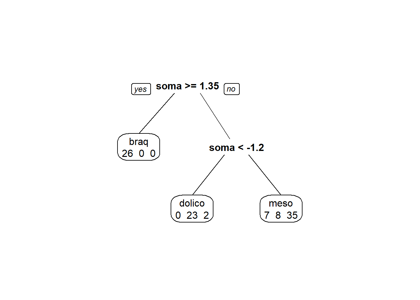
predito = predict(modArvDec01, type = "class")
confusionMatrix(predito, tabfacial$grupo)
## Confusion Matrix and Statistics
##
## Reference
## Prediction braq dolico meso
## braq 26 0 0
## dolico 0 23 2
## meso 7 8 35
##
## Overall Statistics
##
## Accuracy : 0.8317
## 95% CI : (0.7442, 0.8988)
## No Information Rate : 0.3663
## P-Value [Acc > NIR] : < 2.2e-16
##
## Kappa : 0.7444
##
## Mcnemar's Test P-Value : NA
##
## Statistics by Class:
##
## Class: braq Class: dolico Class: meso
## Sensitivity 0.7879 0.7419 0.9459
## Specificity 1.0000 0.9714 0.7656
## Pos Pred Value 1.0000 0.9200 0.7000
## Neg Pred Value 0.9067 0.8947 0.9608
## Prevalence 0.3267 0.3069 0.3663
## Detection Rate 0.2574 0.2277 0.3465
## Detection Prevalence 0.2574 0.2475 0.4950
## Balanced Accuracy 0.8939 0.8567 0.8558#c. É possível ajustar um modelo de regressão logística nesse conjunto de dados? Por quê?
#d. Use o classificador de Fisher para classificar a variável resposta de acordo com variáveis preditoras. Qual é a acurácia do classificador? Ajuste o modelo no conjunto de treino e faça a predição no conjunto de teste.
modFisher01 = lda(grupo ~ soma, data = tabfacial)
predito = predict(modFisher01)
classPred = predito$class
confusionMatrix(classPred, tabfacial$grupo)
## Confusion Matrix and Statistics
##
## Reference
## Prediction braq dolico meso
## braq 29 0 5
## dolico 0 23 2
## meso 4 8 30
##
## Overall Statistics
##
## Accuracy : 0.8119
## 95% CI : (0.7219, 0.8828)
## No Information Rate : 0.3663
## P-Value [Acc > NIR] : < 2.2e-16
##
## Kappa : 0.7157
##
## Mcnemar's Test P-Value : NA
##
## Statistics by Class:
##
## Class: braq Class: dolico Class: meso
## Sensitivity 0.8788 0.7419 0.8108
## Specificity 0.9265 0.9714 0.8125
## Pos Pred Value 0.8529 0.9200 0.7143
## Neg Pred Value 0.9403 0.8947 0.8814
## Prevalence 0.3267 0.3069 0.3663
## Detection Rate 0.2871 0.2277 0.2970
## Detection Prevalence 0.3366 0.2475 0.4158
## Balanced Accuracy 0.9026 0.8567 0.8117#e. Use o classificador de Bayes para classificar a variável resposta de acordo com as variáveis preditoras. Utilize como priori a proporção amostral. Qual é a acurácia do classificador?
library(e1071)
modNaiveBayes01 = naiveBayes(grupo ~ soma, data = tabfacial)
predito = predict(modNaiveBayes01, tabfacial)
confusionMatrix(classPred, tabfacial$grupo)
## Confusion Matrix and Statistics
##
## Reference
## Prediction braq dolico meso
## braq 29 0 5
## dolico 0 23 2
## meso 4 8 30
##
## Overall Statistics
##
## Accuracy : 0.8119
## 95% CI : (0.7219, 0.8828)
## No Information Rate : 0.3663
## P-Value [Acc > NIR] : < 2.2e-16
##
## Kappa : 0.7157
##
## Mcnemar's Test P-Value : NA
##
## Statistics by Class:
##
## Class: braq Class: dolico Class: meso
## Sensitivity 0.8788 0.7419 0.8108
## Specificity 0.9265 0.9714 0.8125
## Pos Pred Value 0.8529 0.9200 0.7143
## Neg Pred Value 0.9403 0.8947 0.8814
## Prevalence 0.3267 0.3069 0.3663
## Detection Rate 0.2871 0.2277 0.2970
## Detection Prevalence 0.3366 0.2475 0.4158
## Balanced Accuracy 0.9026 0.8567 0.8117#f. Use o classificador knn para classificar a variável resposta de acordo com a variável preditora. Utilize k = 1,3,5. Ajuste o modelo no conjunto de treino e faça a predição no conjunto de teste.
modKnn1_01 = knn3(grupo ~ soma, data = tabfacial, k = 1)
predito = predict(modKnn1_01, tabfacial, type = "class")
confusionMatrix(classPred, tabfacial$grupo)
## Confusion Matrix and Statistics
##
## Reference
## Prediction braq dolico meso
## braq 29 0 5
## dolico 0 23 2
## meso 4 8 30
##
## Overall Statistics
##
## Accuracy : 0.8119
## 95% CI : (0.7219, 0.8828)
## No Information Rate : 0.3663
## P-Value [Acc > NIR] : < 2.2e-16
##
## Kappa : 0.7157
##
## Mcnemar's Test P-Value : NA
##
## Statistics by Class:
##
## Class: braq Class: dolico Class: meso
## Sensitivity 0.8788 0.7419 0.8108
## Specificity 0.9265 0.9714 0.8125
## Pos Pred Value 0.8529 0.9200 0.7143
## Neg Pred Value 0.9403 0.8947 0.8814
## Prevalence 0.3267 0.3069 0.3663
## Detection Rate 0.2871 0.2277 0.2970
## Detection Prevalence 0.3366 0.2475 0.4158
## Balanced Accuracy 0.9026 0.8567 0.8117modKnn3_01 = knn3(grupo ~ soma, data = tabfacial, k = 3)
predito = predict(modKnn3_01, tabfacial, type = "class")
confusionMatrix(classPred, tabfacial$grupo)## Confusion Matrix and Statistics
##
## Reference
## Prediction braq dolico meso
## braq 29 0 5
## dolico 0 23 2
## meso 4 8 30
##
## Overall Statistics
##
## Accuracy : 0.8119
## 95% CI : (0.7219, 0.8828)
## No Information Rate : 0.3663
## P-Value [Acc > NIR] : < 2.2e-16
##
## Kappa : 0.7157
##
## Mcnemar's Test P-Value : NA
##
## Statistics by Class:
##
## Class: braq Class: dolico Class: meso
## Sensitivity 0.8788 0.7419 0.8108
## Specificity 0.9265 0.9714 0.8125
## Pos Pred Value 0.8529 0.9200 0.7143
## Neg Pred Value 0.9403 0.8947 0.8814
## Prevalence 0.3267 0.3069 0.3663
## Detection Rate 0.2871 0.2277 0.2970
## Detection Prevalence 0.3366 0.2475 0.4158
## Balanced Accuracy 0.9026 0.8567 0.8117modKnn5_01 = knn3(grupo ~ soma, data = tabfacial, k = 5)
predito = predict(modKnn5_01, tabfacial, type = "class")
confusionMatrix(classPred, tabfacial$grupo)## Confusion Matrix and Statistics
##
## Reference
## Prediction braq dolico meso
## braq 29 0 5
## dolico 0 23 2
## meso 4 8 30
##
## Overall Statistics
##
## Accuracy : 0.8119
## 95% CI : (0.7219, 0.8828)
## No Information Rate : 0.3663
## P-Value [Acc > NIR] : < 2.2e-16
##
## Kappa : 0.7157
##
## Mcnemar's Test P-Value : NA
##
## Statistics by Class:
##
## Class: braq Class: dolico Class: meso
## Sensitivity 0.8788 0.7419 0.8108
## Specificity 0.9265 0.9714 0.8125
## Pos Pred Value 0.8529 0.9200 0.7143
## Neg Pred Value 0.9403 0.8947 0.8814
## Prevalence 0.3267 0.3069 0.3663
## Detection Rate 0.2871 0.2277 0.2970
## Detection Prevalence 0.3366 0.2475 0.4158
## Balanced Accuracy 0.9026 0.8567 0.8117#g. Use naive Bayes para classificar a variável resposta de acordo com as variáveis preditoras. Ajuste o modelo no conjunto de treino e faça a predição no conjunto de teste
library(e1071)
modNaiveBayes01 = naiveBayes(grupo ~ soma, data = tabfacial)
predito = predict(modNaiveBayes01, tabfacial)
confusionMatrix(classPred, tabfacial$grupo)
## Confusion Matrix and Statistics
##
## Reference
## Prediction braq dolico meso
## braq 29 0 5
## dolico 0 23 2
## meso 4 8 30
##
## Overall Statistics
##
## Accuracy : 0.8119
## 95% CI : (0.7219, 0.8828)
## No Information Rate : 0.3663
## P-Value [Acc > NIR] : < 2.2e-16
##
## Kappa : 0.7157
##
## Mcnemar's Test P-Value : NA
##
## Statistics by Class:
##
## Class: braq Class: dolico Class: meso
## Sensitivity 0.8788 0.7419 0.8108
## Specificity 0.9265 0.9714 0.8125
## Pos Pred Value 0.8529 0.9200 0.7143
## Neg Pred Value 0.9403 0.8947 0.8814
## Prevalence 0.3267 0.3069 0.3663
## Detection Rate 0.2871 0.2277 0.2970
## Detection Prevalence 0.3366 0.2475 0.4158
## Balanced Accuracy 0.9026 0.8567 0.8117#i. Use svm para fazer para classificar a variável resposta de acordo com as variáveis preditoras. Ajuste o modelo no conjunto de treino e faça a predição no conjunto de teste.
modSVM01 = svm(grupo ~ soma, data = tabfacial, kernel = "linear")

predito = predict(modSVM01, type = "class")
confusionMatrix(classPred, tabfacial$grupo)
## Confusion Matrix and Statistics
##
## Reference
## Prediction braq dolico meso
## braq 29 0 5
## dolico 0 23 2
## meso 4 8 30
##
## Overall Statistics
##
## Accuracy : 0.8119
## 95% CI : (0.7219, 0.8828)
## No Information Rate : 0.3663
## P-Value [Acc > NIR] : < 2.2e-16
##
## Kappa : 0.7157
##
## Mcnemar's Test P-Value : NA
##
## Statistics by Class:
##
## Class: braq Class: dolico Class: meso
## Sensitivity 0.8788 0.7419 0.8108
## Specificity 0.9265 0.9714 0.8125
## Pos Pred Value 0.8529 0.9200 0.7143
## Neg Pred Value 0.9403 0.8947 0.8814
## Prevalence 0.3267 0.3069 0.3663
## Detection Rate 0.2871 0.2277 0.2970
## Detection Prevalence 0.3366 0.2475 0.4158
## Balanced Accuracy 0.9026 0.8567 0.8117#j. Use uma rede neural para classificar a variável resposta de acordo com as variáveis preditoras. Ajuste o modelo no conjunto de treino e faça a predição no conjunto de teste.
library(neuralnet)

modRedNeural01 = neuralnet(grupo ~ soma, data = tabfacial, hidden = c(2,4,3))
plot(modRedNeural01)

ypred = neuralnet::compute(modRedNeural01, tabfacial)
yhat = ypred$net.result
#Ajustando os modelos
library(caret)
trControl <- trainControl(method = "LOOCV")

fit <- train(sexo ~ soma, method = "glm", data = tabfacial,
             trControl = trControl, metric = "Accuracy")
fit <- train(sexo ~ soma, method = "lda", data = tabfacial, prior = c(0.5, 0.5),
             trControl = trControl, metric = "Accuracy")
fit <- train(sexo ~ soma, method = "lda", data = tabfacial, prior = c(0.65, 0.35),
             trControl = trControl, metric = "Accuracy")
fit <- train(sexo ~ soma, method = "knn", data = tabfacial,
             tuneGrid = expand.grid(k = 1:5),
             trControl = trControl, metric = "Accuracy")
totalAcerto = 0
for (i in 1:nrow(tabfacial)){
    treino = tabfacial[-i,]
    teste = tabfacial[i,]
    modelo = svm(grupo ~ soma, data = treino)
    predito = predict(modelo, newdata = teste,  type = "class")
    if(predito == teste$sexo[1])  totalAcerto = totalAcerto+1
}
2.1.4 Agrupamento:
#Considere os dados a seguir do consumo alimentar médio de diferentes tipos de alimentos para famílias classificadas de acordo com o número de filhos (2, 3, 4 ou 5) e principal área de trabalho (MA: Setor de Trabalho Manual, EM: Empregados do Setor Público ou CA: Cargos Administrativos)
#Um código no R para o conjunto de dados é dado a seguir: #library(tibble) #dados = tibble(AreaTrabalho = as.factor(rep(c(“MA”, “EM”, “CA”), 4)), # Filhos = as.factor(rep(2:5, each = 3)), # Paes = c(332, 293, 372, 406, 386, 438, 534, 460, 385, 655, 584, 515), # Vegetais = c(428, 559, 767, 563, 608, 843, 660, 699, 789, 776, 995, 1097), # Frutas = c(354, 388, 562, 341, 396, 689, 367, 484, 621, 423, 548, 887), # Carnes = c(1437,1527,1948,1507,1501,2345,1620,1856,2366,1848,2056,2630), # Aves = c(526, 567, 927, 544, NA, 1148,638, 762, 1149,759, 893, 1167), # Leite = c(247, 239, 235, 324, 319, 243, 414, 400, 304, 495, 518, 561), # Alcoolicos = c(427, 258, 433, 407, 363, 341, 407, 416, 282, 486, 319, 284))
library(tibble)
dados = tibble(AreaTrabalho = as.factor(rep(c("MA", "EM", "CA"), 4)),
 Filhos = as.factor(rep(2:5, each = 3)),
 Paes = c(332, 293, 372, 406, 386, 438, 534, 460, 385, 655, 584, 515),
 Vegetais = c(428, 559, 767, 563, 608, 843, 660, 699, 789, 776, 995, 1097),
 Frutas = c(354, 388, 562, 341, 396, 689, 367, 484, 621, 423, 548, 887),
 Carnes = c(1437,1527,1948,1507,1501,2345,1620,1856,2366,1848,2056,2630),
 Aves = c(526, 567, 927, 544, NA, 1148,638, 762, 1149,759, 893, 1167),
 Leite = c(247, 239, 235, 324, 319, 243, 414, 400, 304, 495, 518, 561),
 Alcoolicos = c(427, 258, 433, 407, 363, 341, 407, 416, 282, 486, 319, 284))
#a. Utilize regressão linear para predizer o dado faltante em Aves.
library("e1071")
x <- dados
y <- dados$Aves
N = nrow(x)
baseTreino <- sample(1:N, N*0.75, FALSE)
modeloNB <- naiveBayes(y[baseTreino]~., data = x[baseTreino,])
probsTeste <- predict(modeloNB, x[-baseTreino,], type = "raw")
head(round(probsTeste,3),4)
## 526 544 567 759 762 893 1149 1167
## [1,] NA NA NA NA NA NA NA NA
## [2,] NA NA NA NA NA NA NA NA
## [3,] NA NA NA NA NA NA NA NAclassesTeste <- predict(modeloNB, x[-baseTreino,], type = "class")
head(classesTeste)## factor(0)
## Levels: 526 544 567 759 762 893 1149 1167#b. Faça uma análise de agrupamento com as variáveis numéricas. Compare vários métodos hierárquicos, combinando com os tipos de distâncias. Compare também com o método kmédias.
x = dados[,2:6]
x
## # A tibble: 12 × 5
## Filhos Paes Vegetais Frutas Carnes
## <fct> <dbl> <dbl> <dbl> <dbl>
## 1 2 332 428 354 1437
## 2 2 293 559 388 1527
## 3 2 372 767 562 1948
## 4 3 406 563 341 1507
## 5 3 386 608 396 1501
## 6 3 438 843 689 2345
## 7 4 534 660 367 1620
## 8 4 460 699 484 1856
## 9 4 385 789 621 2366
## 10 5 655 776 423 1848
## 11 5 584 995 548 2056
## 12 5 515 1097 887 2630km1 = kmeans(x, 4)
km1## K-means clustering with 4 clusters of sizes 1, 3, 5, 3
##
## Cluster means:
## Filhos Paes Vegetais Frutas Carnes
## 1 5.000000 584.0000 995.0000 548.0000 2056.0
## 2 3.666667 495.6667 747.3333 489.6667 1884.0
## 3 2.800000 390.2000 563.6000 369.2000 1518.4
## 4 4.000000 446.0000 909.6667 732.3333 2447.0
##
## Clustering vector:
## [1] 3 3 2 3 3 4 3 2 4 2 1 4
##
## Within cluster sum of squares by cluster:
## [1] 0.00 61386.67 83014.80 151295.33
## (between_SS / total_SS = 88.4 %)
##
## Available components:
##
## [1] "cluster" "centers" "totss" "withinss" "tot.withinss" "betweenss" "size" "iter" "ifault"