Chapter 5 Analisando dataframe de Ação

5.1 Análise descritiva

Coletando os dados

library(lubridate)
library(tidyverse)
series = read_excel("dados/03 B1 ESTATISTICAS DESC E REGRESSAO.xlsx", sheet = 2, n_max = 1)

## New names:
## • `44824` -> `44824...2`
## • `44824` -> `44824...4`
## • `44824` -> `44824...6`
## • `44824` -> `44824...8`
## • `44824` -> `44824...10`
## • `44824` -> `44824...12`
## • `44824` -> `44824...14`
## • `44824` -> `44824...16`
## • `44824` -> `44824...18`
## • `44824` -> `44824...20`

nomes = names(series)[seq(1,20,2)]
series = read_excel("dados/03 B1 ESTATISTICAS DESC E REGRESSAO.xlsx", sheet = 2, skip = 1)

## New names:
## • `Date` -> `Date...1`
## • `Close` -> `Close...2`
## • `Date` -> `Date...3`
## • `Close` -> `Close...4`
## • `Date` -> `Date...5`
## • `Close` -> `Close...6`
## • `Date` -> `Date...7`
## • `Close` -> `Close...8`
## • `Date` -> `Date...9`
## • `Close` -> `Close...10`
## • `Date` -> `Date...11`
## • `Close` -> `Close...12`
## • `Date` -> `Date...13`
## • `Close` -> `Close...14`
## • `Date` -> `Date...15`
## • `Close` -> `Close...16`
## • `Date` -> `Date...17`
## • `Close` -> `Close...18`
## • `Date` -> `Date...19`
## • `Close` -> `Close...20`

names(series)[seq(1,20,2)] = paste0("DATA_", nomes)
names(series)[seq(2,20,2)] = nomes
series

## # A tibble: 3,147 × 20
##    DATA_ELET3          ELET3 DATA_ITUB4          ITUB4 DATA_ITSA4          ITSA4 DATA_PETR4          PETR4 DATA_NUBR33         NUBR33 DATA_MGLU3          MGLU3 DATA_BBDC4          BBDC4
##    <dttm>              <dbl> <dttm>              <dbl> <dttm>              <dbl> <dttm>              <dbl> <dttm>               <dbl> <dttm>              <dbl> <dttm>              <dbl>
##  1 2010-01-04 16:56:00  37.4 2010-01-04 16:56:00  20.1 2010-01-04 16:56:00  8.05 2010-01-04 16:56:00  37.3 2021-12-09 16:56:00  10.0  2011-05-02 16:56:00  0.51 2010-01-04 16:56:00  12.2
##  2 2010-01-05 16:56:00  37.1 2010-01-05 16:56:00  20.2 2010-01-05 16:56:00  8.02 2010-01-05 16:56:00  37   2021-12-10 16:56:00  11.5  2011-05-03 16:56:00  0.51 2010-01-05 16:56:00  12.1
##  3 2010-01-06 16:56:00  36.6 2010-01-06 16:56:00  20.0 2010-01-06 16:56:00  7.92 2010-01-06 16:56:00  37.5 2021-12-13 18:00:00  10.6  2011-05-04 16:56:00  0.52 2010-01-06 16:56:00  12  
##  4 2010-01-07 16:56:00  37.4 2010-01-07 16:56:00  19.8 2010-01-07 16:56:00  7.88 2010-01-07 16:56:00  37.2 2021-12-14 18:00:00   9.25 2011-05-05 16:56:00  0.51 2010-01-07 16:56:00  12.0
##  5 2010-01-08 16:56:00  38.1 2010-01-08 16:56:00  19.5 2010-01-08 16:56:00  7.82 2010-01-08 16:56:00  37.0 2021-12-15 18:00:00   9.54 2011-05-06 16:56:00  0.51 2010-01-08 16:56:00  12.0
##  6 2010-01-11 16:56:00  37.5 2010-01-11 16:56:00  19.4 2010-01-11 16:56:00  7.79 2010-01-11 16:56:00  36.8 2021-12-16 18:00:00   9.49 2011-05-10 16:56:00  0.5  2010-01-11 16:56:00  12.0
##  7 2010-01-12 16:56:00  37.1 2010-01-12 16:56:00  19.2 2010-01-12 16:56:00  7.79 2010-01-12 16:56:00  36.4 2021-12-17 18:00:00   8.95 2011-05-11 16:56:00  0.51 2010-01-12 16:56:00  12  
##  8 2010-01-13 16:56:00  37.5 2010-01-13 16:56:00  19.2 2010-01-13 16:56:00  7.77 2010-01-13 16:56:00  36.3 2021-12-20 18:00:00   8.5  2011-05-12 16:56:00  0.51 2010-01-13 16:56:00  12.1
##  9 2010-01-14 16:56:00  36.9 2010-01-14 16:56:00  19.0 2010-01-14 16:56:00  7.66 2010-01-14 16:56:00  35.7 2021-12-21 18:00:00   8.7  2011-05-13 16:56:00  0.51 2010-01-14 16:56:00  11.8
## 10 2010-01-15 16:56:00  35.6 2010-01-15 16:56:00  18.7 2010-01-15 16:56:00  7.47 2010-01-15 16:56:00  35.8 2021-12-22 18:00:00   8.54 2011-05-17 16:56:00  0.5  2010-01-15 16:56:00  11.6
## # … with 3,137 more rows, and 6 more variables: DATA_VALE3 <dttm>, VALE3 <dbl>, DATA_BBAS3 <dttm>, BBAS3 <dbl>, DATA_LREN3 <dttm>, LREN3 <dbl>

for (i in seq(1,20,2)) {
  series[[i]] = as.Date(series[[i]])
}

plot(x=series$DATA_ELET3, y= series$ELET3, type = "l", xlab = "Tempo (dias)", ylab = "Preço fechamento (R$)",  main = "Performance de algumas ações ao longo do tempo", ylim = c(0, 60) )
lines(x=series$DATA_ITUB4, y= series$ITUB4, col = 2)
lines(x=series$DATA_PETR4, y= series$PETR4, col = 3)
lines(x=series$DATA_NUBR33, y= series$NUBR33, col = 4)
legend("topleft", legend = c("ELET3", "ITUB4", "PETR4", "NUBR33"), fill = c(1,2,3,4))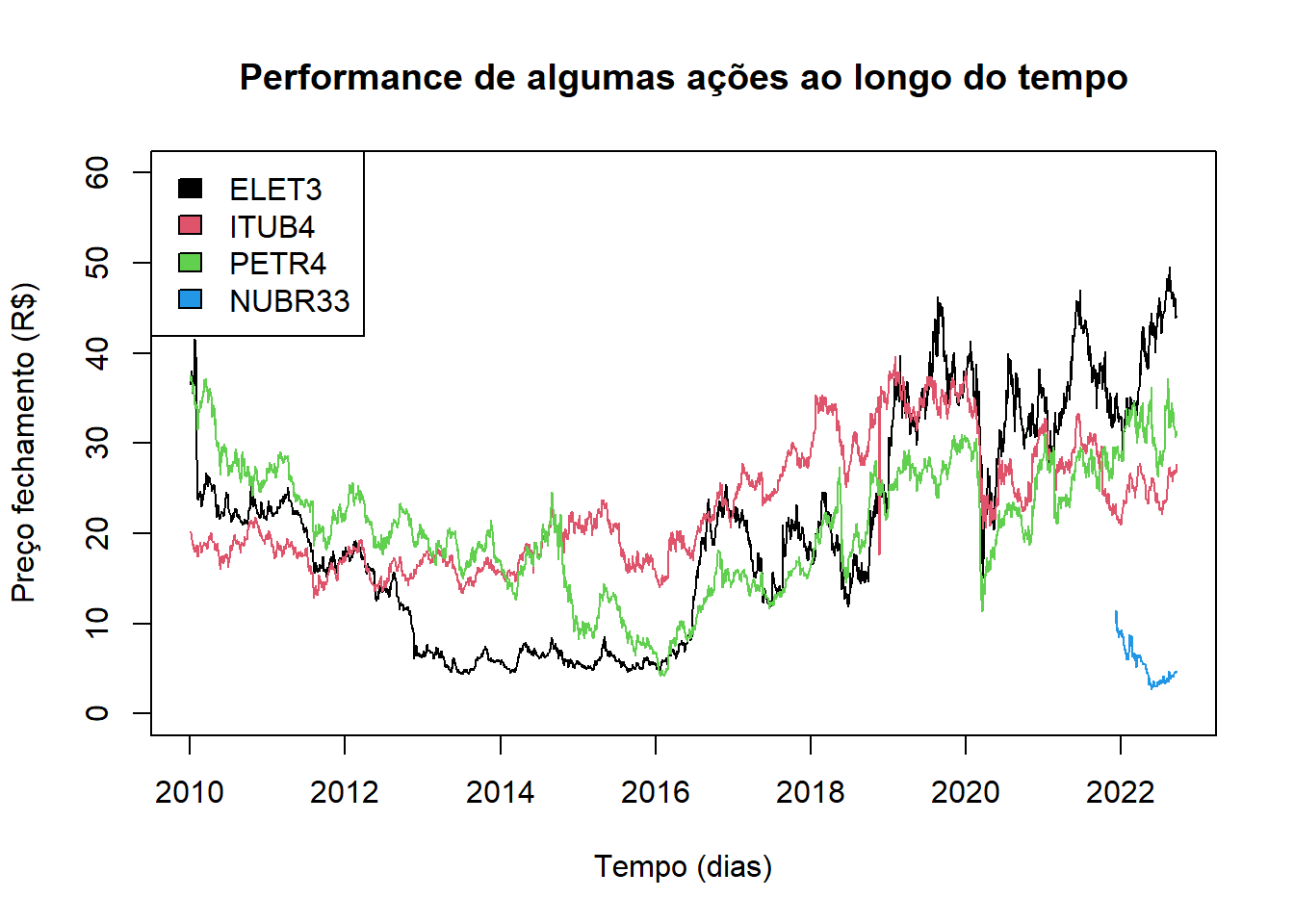

## Selecionando um tipo de Ação para Analise Descritiva

dataInicial = as.Date("2020-01-01")
dataFinal  = as.Date("2021-01-01")
subConjunto = filter(series, DATA_ITUB4 >= dataInicial & DATA_ITUB4 <= dataFinal)

Apresentado os dados selecionado em um grafico

Data = subConjunto$DATA_ITUB4
Ser = subConjunto$ITUB4
media = mean(Ser, na.rm = T)
media

## [1] 26.91806

desvio = sd(Ser, na.rm = T)
desvio

## [1] 4.125498

plot(x=Data, y= Ser, type = "l", xlab = "Tempo (dias)", ylab = "Preço fechamento (R$)")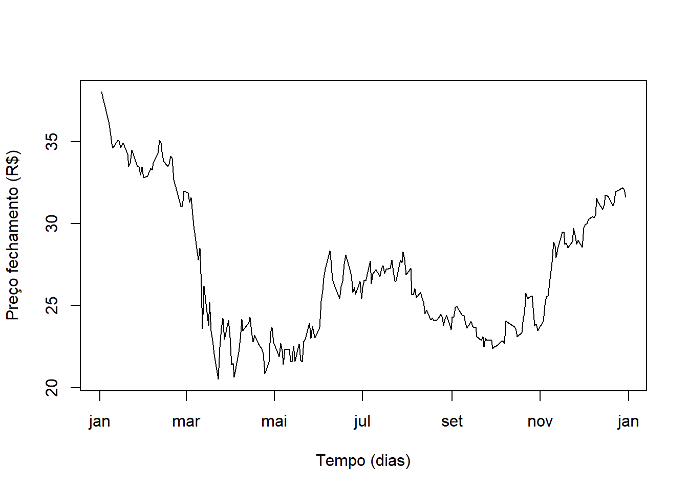

Apresentado os dados selecionado em um grafico

plot(Ser ~ Data, type = "l", xlab = "Tempo (dias)", ylab = "Preço fechamento (R$)", ylim = c(-10, 80))
abline(h = media)
abline(h = media + 1*desvio, col = 2, lwd = 2)
abline(h = media - 1*desvio, col = 2, lwd = 2)
abline(h = media + 2*desvio, col = 3, lwd = 2)
abline(h = media - 2*desvio, col = 3, lwd = 2)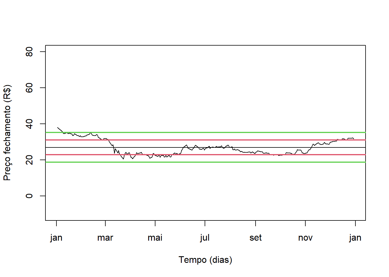

Apresentado os dados selecionado em um grafico

#caixa = boxplot(Ser ~ Data, add = T)
#caixa
#limSup = caixa$stats[5,1]
#Q3 = caixa$stats[4,1]
#Q2 = caixa$stats[3,1]
#Q1 = caixa$stats[2,1]
#limInf = caixa$stats[1,1]

#plot(Ser ~ Data, type = "l", xlab = "Tempo (dias)", ylab = "Preço fechamento (R$)", ylim = c(-0, 40))
#abline(h = Q2)
#abline(h = Q3, col = 2, lwd = 2)
#abline(h = Q1, col = 2, lwd = 2)
#abline(h = limSup, col = 3, lwd = 2)
#abline(h = limInf, col = 3, lwd = 2)