B Solutions to formative assessment

library(tidyverse)
library(magrittr)

B.1 Question 1

Load the dataset into R as a tibble and check your variables are what you expect them to be using the command str

Make sure you have set your working directory and saved the file here.

chd <- read.csv("CHD.csv")

str(chd)

## 'data.frame':    462 obs. of  10 variables:
##  $ sbp      : int  160 144 118 170 134 132 142 114 114 132 ...
##  $ tobacco  : num  12 0.01 0.08 7.5 13.6 6.2 4.05 4.08 0 0 ...
##  $ ldl      : num  5.73 4.41 3.48 6.41 3.5 6.47 3.38 4.59 3.83 5.8 ...
##  $ adiposity: num  23.1 28.6 32.3 38 27.8 ...
##  $ famhist  : chr  "Present" "Absent" "Present" "Present" ...
##  $ typea    : int  49 55 52 51 60 62 59 62 49 69 ...
##  $ obesity  : num  25.3 28.9 29.1 32 26 ...
##  $ alcohol  : num  97.2 2.06 3.81 24.26 57.34 ...
##  $ age      : int  52 63 46 58 49 45 38 58 29 53 ...
##  $ chd      : int  1 1 0 1 1 0 0 1 0 1 ...

B.2 Question 2

Change the variable name ‘obesity’ to ‘BMI’ and find the mean BMI of the individuals in the CHD dataset.

There are a few ways to do this, a base R solution would be like this

colnames(chd)[7] <- "bmi"

Or you could use dplyr

chd <- chd %>%
  rename(bmi = "obesity")

Then calculate the mean

mean(chd$bmi)

## [1] 26.04411

B.3 Question 3

Plot a histogram of the distribution of the BMI of the individuals in the CHD dataset (Use 25 breaks in your histogram). Make sure you have named the axes of your histogram and added a title.

hist(chd$bmi, breaks = 25, xlab = "BMI (kg/m^2)", main = "Distribution of BMI")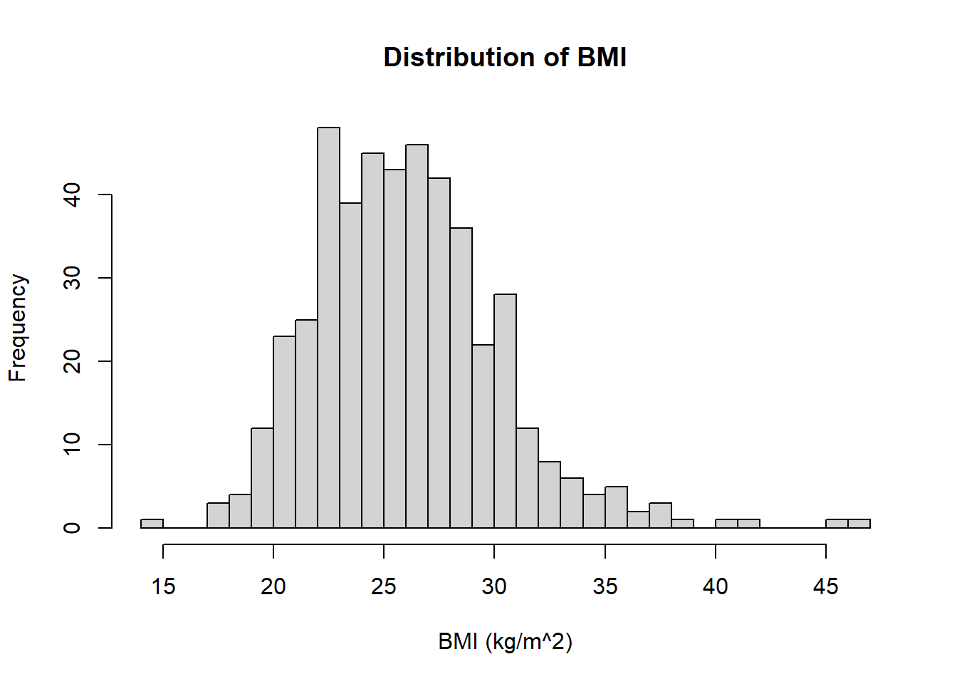

B.4 Question 4

Create a boxplot for the distribution of BMI variable.

boxplot(chd$bmi, horizontal = TRUE, xlab = "BMI (kg/m^2)")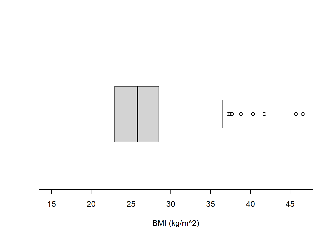

B.5 Question 5

Find the function to give the interquartile range (explained below) of the variable tobacco and interpret the results.

IQR(chd$tobacco)

## [1] 5.4475

B.6 Question 6

Create a new data set called y which contains only the first ten entries of the CHD data set.

Again there are different ways to do this, in base R:

y <- chd[1:10, ]

Or using the tidyverse:

y <- chd %>%
  slice(1:10)

B.7 Question 7

Calculate the standard deviation for the systolic blood pressure variable using the operator %$%.

chd %$%
  sd(sbp)

## [1] 20.49632

B.8 Question 8

Use ggplot to plot tobacco vs sbp, coloured red if they have chd and green if they don’t. Add in a line of best fit for each of the groups, with the relevant colour.

ggplot(data = chd) +
  geom_point(mapping = aes(y = tobacco, x = sbp,  colour = as.factor(chd))) +
  geom_smooth(aes(y = tobacco, x = sbp, group = as.factor(chd), colour = as.factor(chd)), 
              method = "lm", se = FALSE) +
  labs(title = "Systolic Blood Pressure vs Tobacco Use", 
       x = "Systolic Blood Pressure (mmHg)", 
       y = "Tobacco Use") +
  scale_colour_manual(aesthetics = "colour", values = c("darkgreen", "red"), 
                      label = c("No", "Yes"), name = "CHD") +
  theme_minimal()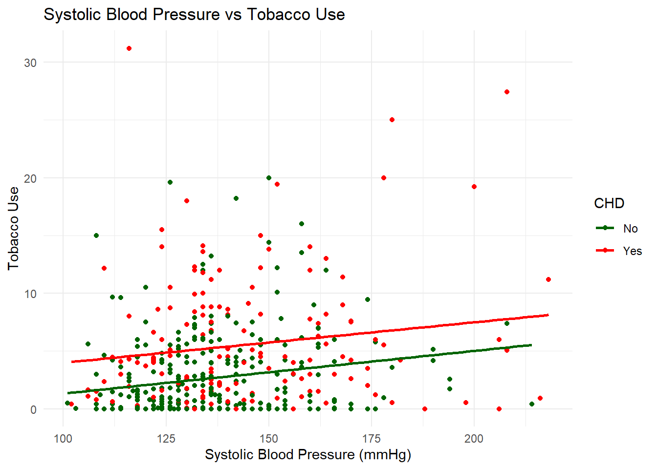

B.9 Question 9

Use the filter function to subset the data to those with chd and a BMI between 18.5 and 25. Then use the arrange function to order them by tobacco intake.

sub <- chd %>%
  filter(chd == 1) %>%
  filter(bmi >= 18.5 & bmi < 25) %>%
  arrange(tobacco)

dim(sub)

## [1] 54 10

B.10 Question 10

Write a function which does the same as above where you can enter the bounds of the BMI that you are interested in, i.e. if you call the function data_subset_BMI then the command data_subset_BMI(18.5,25) produces the same as your answer to question 9.

data_subset_bmi <- function(x, y){
  chd %>%
    filter(chd == "1") %>%
    filter(bmi >= x & bmi < y) %>%
    arrange(tobacco)
}

sub_2 <- data_subset_bmi(18.5, 25)
dim(sub_2)

## [1] 54 10