Chapter 3 Data
The data used for this tutorial were simulated in R to loosely represent a cohort of XYZ university (XYZ-U) students. As accurate counts and frequencies of the predictors were not available (see: simulated data), “best guesses” were employed where necessary. In a fictional scenario, XYZ university has decided to add a Math Achievement Test as a graduation requirement: students must take this test the semester they anticipate graduating as a measure of their Math Achievement at XYZ university. This is a low stakes assessment and there are no penalties for low scores. XYZ-U, recognizing that many factors may play into how well a student does on this test, wants to consider the role different math teachers play as well as some student-level predictors. Not wanting this to hold any penalty towards teachers either, XYZ-U has assigned each teacher an anonymous ID and associated it with the years of experience. XYZ-U is additionally considering what teacher qualities help students be more successful, with the idea of offering more professional development in those areas. Currently, the only teacher-level predictor available is number of years of experience of the instructor.
The university hopes to answer the following research questions: RQ1: Do teacher characteristics influence student math scores? RQ2: What student characteristics predict math scores? RQ3: Does more teacher experience lead to better student outcomes?
The predictors are listed in the table below, along with a brief description.
| Predictor | Description |
|---|---|
| MathAch | Mach Achievement; outcome variable, score on a (fictional) math test given to students |
| S_ID | Student ID; a single number representation of students, from 1 to 5200 |
| SAT_M | SAT math score; ranges from 200-800 and represents the SAT math score of students prior to entering JMU. |
| S_gend | Student gender; a non-binary gender indicator with 0 = female, 1 = male, and 2 = other/nonbinary/fluid |
| female, NB | Dummy coded student gender, since gender is categorical. Male is the reference |
| S_SES | Student SES; values range from 2-29 |
| num_tchrs | Number of teachers; the number of math teachers a student had at JMU |
| phys | Physics; if a student took physics or not, with 0 = no and 1 = yes |
| phys_tchr | Physics teacher; if a student took physics, the ID of the teacher they had (ranging from 1 – 22) |
| tchr1-tchr12 | Teachers 1 through 12; teacher IDs (ranging from 1-56) of teachers students had. If a student had less than 12 teachers, teacher ID = 0 |
| w1-w12 | Weights; these represent the amount of time spent with each teacher. Values can range from 1 (only had one teacher) to 0.083 (had 12 teachers) |
| t1_exp-t12_exp | Teacher experience; Given the compact nature of this dataset, the experience of the first through twelfth teachers of each student is given in years. |
3.1 Compact vs. wide forms
The data are in a .cvs file in “compact” form, as opposed to “wide” form. Compact form contains two different sets of variables: one set for the first through twelfth teacher to instruct each student and another set represent the multiple membership weight variables. Wide form would have the same information, but in only one set of variables representing the individual teacher IDs and the proportion of time each teacher spent instructing each student in the cells (see tables below).
3.1.1 Compact
In compact form, there is a set of variables for the max number of level 2 units encountered, and another set of variables for the weights. Adding in a level-2 predictor here would only necessitate adding in the appropriate number of columns for the number of level 2 units encountered for that predictor. Using our data as an example, we have teacher experience as a level 2 predictor, and 12 possible teacher encounters. To add in teacher experience, we would add in 12 columns, t_exp1-t_exp12, which would populate with the appropriate experience for the teacher the student had. The weight would be calculated via the weight columns.
| Student | Teacher.1 | Teacher.2 | Teacher.3 | w1 | w2 | w3 |
|---|---|---|---|---|---|---|
| 1 | 2 | 4 | 1 | 0.33 | 0.33 | 0.33 |
| 2 | 2 | 3 | 1 | 0.33 | 0.33 | 0.33 |
| 3 | 3 | 1 | 4 | 0.33 | 0.33 | 0.33 |
| 4 | 0 | 3 | 0 | 0.00 | 1.00 | 0.00 |
| 5 | 1 | 0 | 0 | 1.00 | 0.00 | 0.00 |
| 6 | 0 | 1 | 3 | 0.00 | 0.50 | 0.50 |
| 7 | 0 | 1 | 2 | 0.00 | 0.50 | 0.50 |
| 8 | 0 | 0 | 1 | 0.00 | 0.00 | 1.00 |
| 9 | 1 | 2 | 0 | 0.50 | 0.50 | 0.00 |
| 10 | 4 | 0 | 2 | 0.50 | 0.00 | 0.50 |
3.1.2 Wide
While perhaps less evident in this small example, if there were more teacher IDs (56, as in our data for example), but a small number of level 2 units encountered and the associated weights (12 of each in our data), the ‘wide’ descriptor would become more evident. The wide descriptor becomes even more evident when considering level two predictors in the model. In the wide format, every level-2 predictor we add will be calculated across all the level-2 ids. Using our data as an example, we have teacher experience as a level-2 predictor. Adding it in using a wide format would mean including 56 columns for the teacher IDs, with weights in the cell to represent the time each student spent with that teacher. Then, there would be another 56 columns for the teacher experience for each of the teachers, with each of their respective experiences.
| Student | T1 | T2 | T3 | T4 |
|---|---|---|---|---|
| 1 | 0.33 | 0.33 | 0.00 | 0.33 |
| 2 | 0.33 | 0.33 | 0.33 | 0.00 |
| 3 | 0.33 | 0.00 | 0.33 | 0.33 |
| 4 | 0.00 | 0.00 | 1.00 | 0.00 |
| 5 | 1.00 | 0.00 | 0.00 | 0.00 |
| 6 | 0.50 | 0.00 | 0.50 | 0.00 |
| 7 | 0.50 | 0.50 | 0.00 | 0.00 |
| 8 | 1.00 | 0.00 | 0.00 | 0.00 |
| 9 | 0.50 | 0.50 | 0.00 | 0.00 |
| 10 | 0.00 | 0.50 | 0.00 | 0.50 |
While the wide form is less efficient, some programs require the data to be in one form or the other. In this instance, MLwiN using Bayesian routines (what we will be using) requires compact form (Leckie 2013b).
3.2 Examining the Data
The next step is to determine what type of predictors we have and what they look like, as well as if we have a true hierarchical model, a “nesting as nuisance” model, or a non-hierarchical model such as cross-classified or multiple membership models. We will be looking for if students (in this case) belong to one and only one cluster (teachers), which would indicate a hierarchical approach or perhaps a “nesting as nuisance” approach. However, if, as is the case, students belong to multiple clusters, we will be taking a non-hierarchical approach. For this example, we are only considering one cluster, so we will be using a multiple membership design. We can see in the num_tchrs column there are students ranging from having had 1 teacher to 12 teachers, indicating we have a multiple membership column. We could also look at the tchr1 through tchr12 columns, and see there are values in more than one of those - indicating that students have encountered more than one math teacher.
#Read in the data file
StudData <- read.csv("exampledata2.csv")

#See what it looks like
head(StudData)
## X.2 X.1 X S_ID S_gend S_SES num_tchrs phys tchr1 tchr2 tchr3 tchr4 tchr5 tchr6 tchr7 tchr8 tchr9 tchr10 tchr11 tchr12 w1 w2 w3 w4 w5
## 1 1 1 1 1 0 14.880674 3 0 24 32 46 0 0 0 0 0 0 0 0 0 0.33 0.33 0.33 0.00 0
## 2 2 2 2 2 0 14.575710 4 0 30 52 54 18 0 0 0 0 0 0 0 0 0.25 0.25 0.25 0.25 0
## 3 3 3 3 3 1 13.173884 1 0 12 0 0 0 0 0 0 0 0 0 0 0 1.00 0.00 0.00 0.00 0
## 4 4 4 4 4 1 13.065602 2 0 32 30 0 0 0 0 0 0 0 0 0 0 0.50 0.50 0.00 0.00 0
## 5 5 5 5 5 0 16.105715 2 0 3 48 0 0 0 0 0 0 0 0 0 0 0.50 0.50 0.00 0.00 0
## 6 6 6 6 6 1 8.190244 2 1 3 44 0 0 0 0 0 0 0 0 0 0 0.50 0.50 0.00 0.00 0
## w6 w7 w8 w9 w10 w11 w12 Math t10_exp t1_exp t2_exp t3_exp t4_exp t5_exp t6_exp t7_exp t8_exp t9_exp t11_exp t12_exp phys_tchr SAT_M
## 1 0 0 0 0 0 0 0 530.3671 0 9.512710 9.603359 11.08068 0.000000 0 0 0 0 0 0 0 0 795
## 2 0 0 0 0 0 0 0 523.2353 0 10.138500 12.664019 11.33673 4.434515 0 0 0 0 0 0 0 0 693
## 3 0 0 0 0 0 0 0 457.6296 0 12.682655 0.000000 0.00000 0.000000 0 0 0 0 0 0 0 0 706
## 4 0 0 0 0 0 0 0 504.4141 0 9.603359 10.138500 0.00000 0.000000 0 0 0 0 0 0 0 0 654
## 5 0 0 0 0 0 0 0 443.2032 0 9.541097 12.631969 0.00000 0.000000 0 0 0 0 0 0 0 0 419
## 6 0 0 0 0 0 0 0 431.5336 0 9.541097 11.309230 0.00000 0.000000 0 0 0 0 0 0 0 9 416
## female NB
## 1 1 0
## 2 1 0
## 3 0 0
## 4 0 0
## 5 1 0
## 6 0 0summary(StudData)## X.2 X.1 X S_ID S_gend S_SES num_tchrs phys tchr1
## Min. : 1 Min. : 1 Min. : 1 Min. : 1 Min. :0.0000 Min. : 5.657 Min. : 1.000 Min. :0.0000 Min. : 1.00
## 1st Qu.:1301 1st Qu.:1301 1st Qu.:1301 1st Qu.:1301 1st Qu.:0.0000 1st Qu.:11.652 1st Qu.: 1.000 1st Qu.:0.0000 1st Qu.:14.00
## Median :2600 Median :2600 Median :2600 Median :2600 Median :0.0000 Median :12.988 Median : 2.000 Median :0.0000 Median :29.00
## Mean :2600 Mean :2600 Mean :2600 Mean :2600 Mean :0.4708 Mean :12.996 Mean : 2.593 Mean :0.2492 Mean :28.61
## 3rd Qu.:3900 3rd Qu.:3900 3rd Qu.:3900 3rd Qu.:3900 3rd Qu.:1.0000 3rd Qu.:14.353 3rd Qu.: 4.000 3rd Qu.:0.0000 3rd Qu.:43.00
## Max. :5200 Max. :5200 Max. :5200 Max. :5200 Max. :2.0000 Max. :20.249 Max. :12.000 Max. :1.0000 Max. :56.00
## tchr2 tchr3 tchr4 tchr5 tchr6 tchr7 tchr8 tchr9
## Min. : 0.00 Min. : 0.000 Min. : 0.000 Min. : 0.00 Min. : 0.000 Min. : 0.0000 Min. : 0.0000 Min. : 0.0000
## 1st Qu.: 0.00 1st Qu.: 0.000 1st Qu.: 0.000 1st Qu.: 0.00 1st Qu.: 0.000 1st Qu.: 0.0000 1st Qu.: 0.0000 1st Qu.: 0.0000
## Median :14.00 Median : 0.000 Median : 0.000 Median : 0.00 Median : 0.000 Median : 0.0000 Median : 0.0000 Median : 0.0000
## Mean :18.73 Mean : 9.415 Mean : 7.238 Mean : 5.06 Mean : 2.625 Mean : 0.4515 Mean : 0.4065 Mean : 0.3956
## 3rd Qu.:35.00 3rd Qu.:14.000 3rd Qu.: 1.000 3rd Qu.: 0.00 3rd Qu.: 0.000 3rd Qu.: 0.0000 3rd Qu.: 0.0000 3rd Qu.: 0.0000
## Max. :57.00 Max. :57.000 Max. :57.000 Max. :56.00 Max. :57.000 Max. :55.0000 Max. :56.0000 Max. :56.0000
## tchr10 tchr11 tchr12 w1 w2 w3 w4 w5
## Min. : 0.0000 Min. : 0.0000 Min. : 0.0000 Min. :0.0830 Min. :0.0000 Min. :0.00000 Min. :0.00000 Min. :0.00000
## 1st Qu.: 0.0000 1st Qu.: 0.0000 1st Qu.: 0.0000 1st Qu.:0.2500 1st Qu.:0.0000 1st Qu.:0.00000 1st Qu.:0.00000 1st Qu.:0.00000
## Median : 0.0000 Median : 0.0000 Median : 0.0000 Median :0.5000 Median :0.2000 Median :0.00000 Median :0.00000 Median :0.00000
## Mean : 0.3735 Mean : 0.3406 Mean : 0.2996 Mean :0.5784 Mean :0.2424 Mean :0.07666 Mean :0.04988 Mean :0.03008
## 3rd Qu.: 0.0000 3rd Qu.: 0.0000 3rd Qu.: 0.0000 3rd Qu.:1.0000 3rd Qu.:0.5000 3rd Qu.:0.16600 3rd Qu.:0.08300 3rd Qu.:0.00000
## Max. :56.0000 Max. :57.0000 Max. :57.0000 Max. :1.0000 Max. :0.5000 Max. :0.33000 Max. :0.25000 Max. :0.20000
## w6 w7 w8 w9 w10 w11 w12 Math
## Min. :0.00000 Min. :0.000000 Min. :0.00000 Min. :0.00000 Min. :0.000000 Min. :0.0000000 Min. :0.0000000 Min. :283.9
## 1st Qu.:0.00000 1st Qu.:0.000000 1st Qu.:0.00000 1st Qu.:0.00000 1st Qu.:0.000000 1st Qu.:0.0000000 1st Qu.:0.0000000 1st Qu.:396.6
## Median :0.00000 Median :0.000000 Median :0.00000 Median :0.00000 Median :0.000000 Median :0.0000000 Median :0.0000000 Median :442.4
## Mean :0.01458 Mean :0.001487 Mean :0.00124 Mean :0.00112 Mean :0.001035 Mean :0.0009777 Mean :0.0009258 Mean :442.0
## 3rd Qu.:0.00000 3rd Qu.:0.000000 3rd Qu.:0.00000 3rd Qu.:0.00000 3rd Qu.:0.000000 3rd Qu.:0.0000000 3rd Qu.:0.0000000 3rd Qu.:486.1
## Max. :0.16600 Max. :0.142800 Max. :0.12500 Max. :0.11000 Max. :0.100000 Max. :0.0900000 Max. :0.0830000 Max. :614.1
## t10_exp t1_exp t2_exp t3_exp t4_exp t5_exp t6_exp t7_exp
## Min. : 0.0000 Min. : 4.435 Min. : 0.000 Min. : 0.000 Min. : 0.000 Min. : 0.000 Min. : 0.0000 Min. : 0.0000
## 1st Qu.: 0.0000 1st Qu.: 9.300 1st Qu.: 0.000 1st Qu.: 0.000 1st Qu.: 0.000 1st Qu.: 0.000 1st Qu.: 0.0000 1st Qu.: 0.0000
## Median : 0.0000 Median :10.725 Median : 9.112 Median : 0.000 Median : 0.000 Median : 0.000 Median : 0.0000 Median : 0.0000
## Mean : 0.1229 Mean :10.453 Mean : 6.928 Mean : 3.449 Mean : 2.618 Mean : 1.806 Mean : 0.9881 Mean : 0.1677
## 3rd Qu.: 0.0000 3rd Qu.:11.512 3rd Qu.:11.126 3rd Qu.: 9.112 3rd Qu.: 4.435 3rd Qu.: 0.000 3rd Qu.: 0.0000 3rd Qu.: 0.0000
## Max. :14.0426 Max. :14.728 Max. :14.728 Max. :14.728 Max. :14.728 Max. :14.728 Max. :14.7281 Max. :14.7281
## t8_exp t9_exp t11_exp t12_exp phys_tchr SAT_M female NB
## Min. : 0.0000 Min. : 0.0000 Min. : 0.0000 Min. : 0.0000 Min. : 0.00 Min. :200.0 Min. :0.0000 Min. :0.0000
## 1st Qu.: 0.0000 1st Qu.: 0.0000 1st Qu.: 0.0000 1st Qu.: 0.0000 1st Qu.: 0.00 1st Qu.:350.0 1st Qu.:0.0000 1st Qu.:0.0000
## Median : 0.0000 Median : 0.0000 Median : 0.0000 Median : 0.0000 Median : 0.00 Median :500.0 Median :1.0000 Median :0.0000
## Mean : 0.1475 Mean : 0.1378 Mean : 0.1203 Mean : 0.1151 Mean : 2.88 Mean :499.8 Mean :0.5717 Mean :0.0425
## 3rd Qu.: 0.0000 3rd Qu.: 0.0000 3rd Qu.: 0.0000 3rd Qu.: 0.0000 3rd Qu.: 0.00 3rd Qu.:646.2 3rd Qu.:1.0000 3rd Qu.:0.0000
## Max. :13.9805 Max. :14.7281 Max. :14.7281 Max. :14.7281 Max. :22.00 Max. :800.0 Max. :1.0000 Max. :1.0000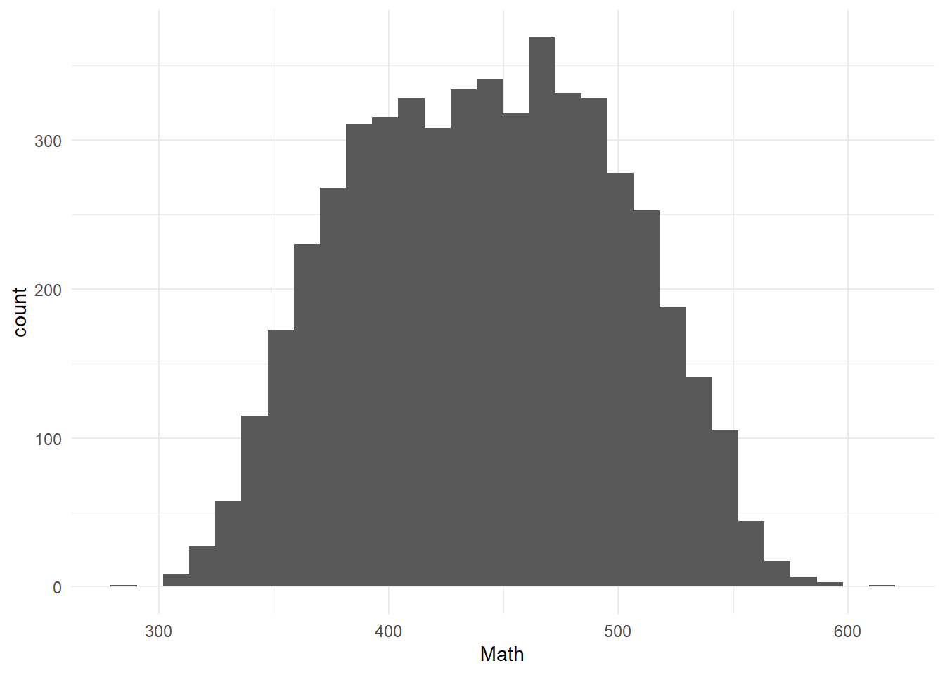
Figure 3.1: Distribution of the outcome (Math)
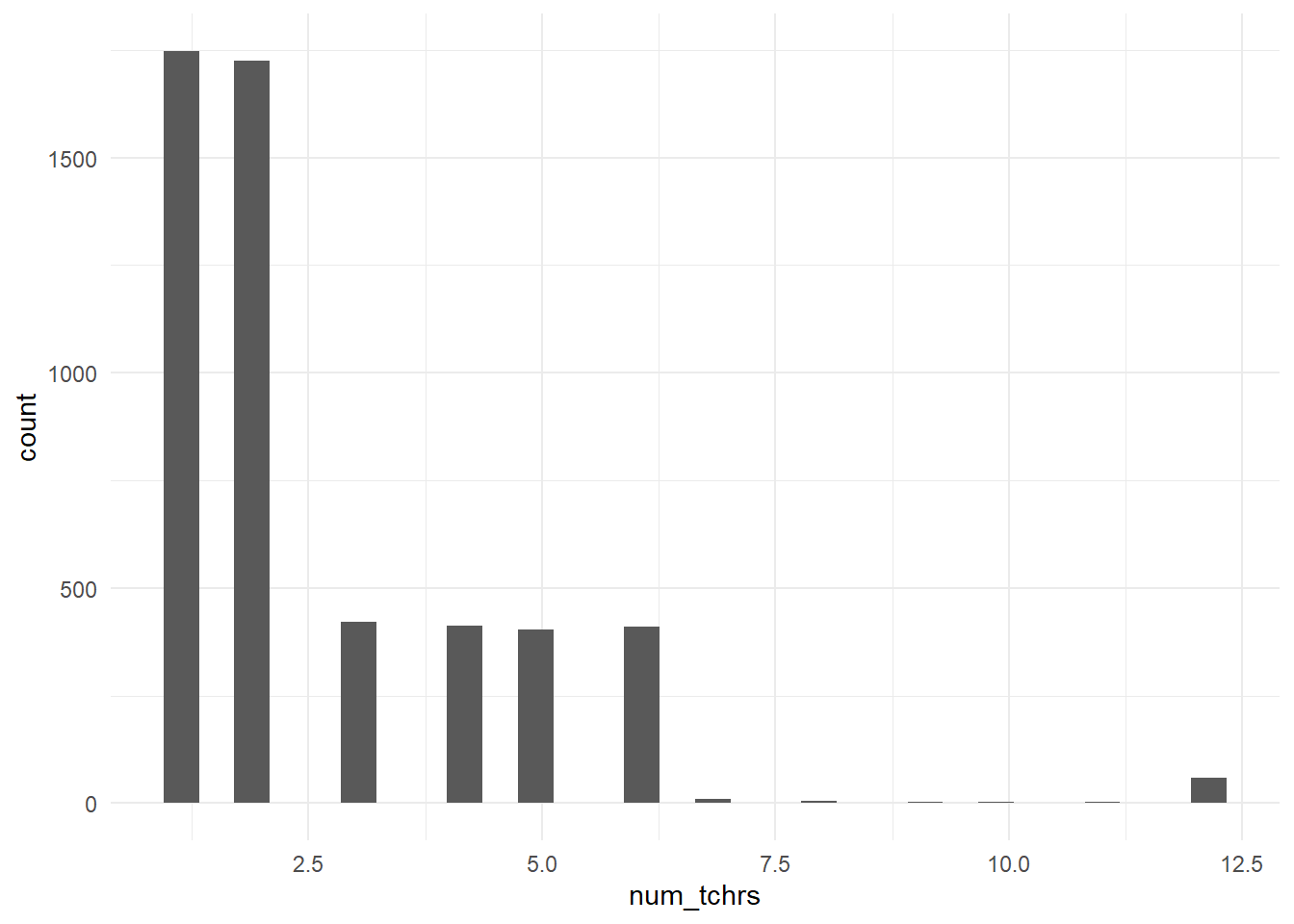
Figure 3.2: Distribution of the number of teachers
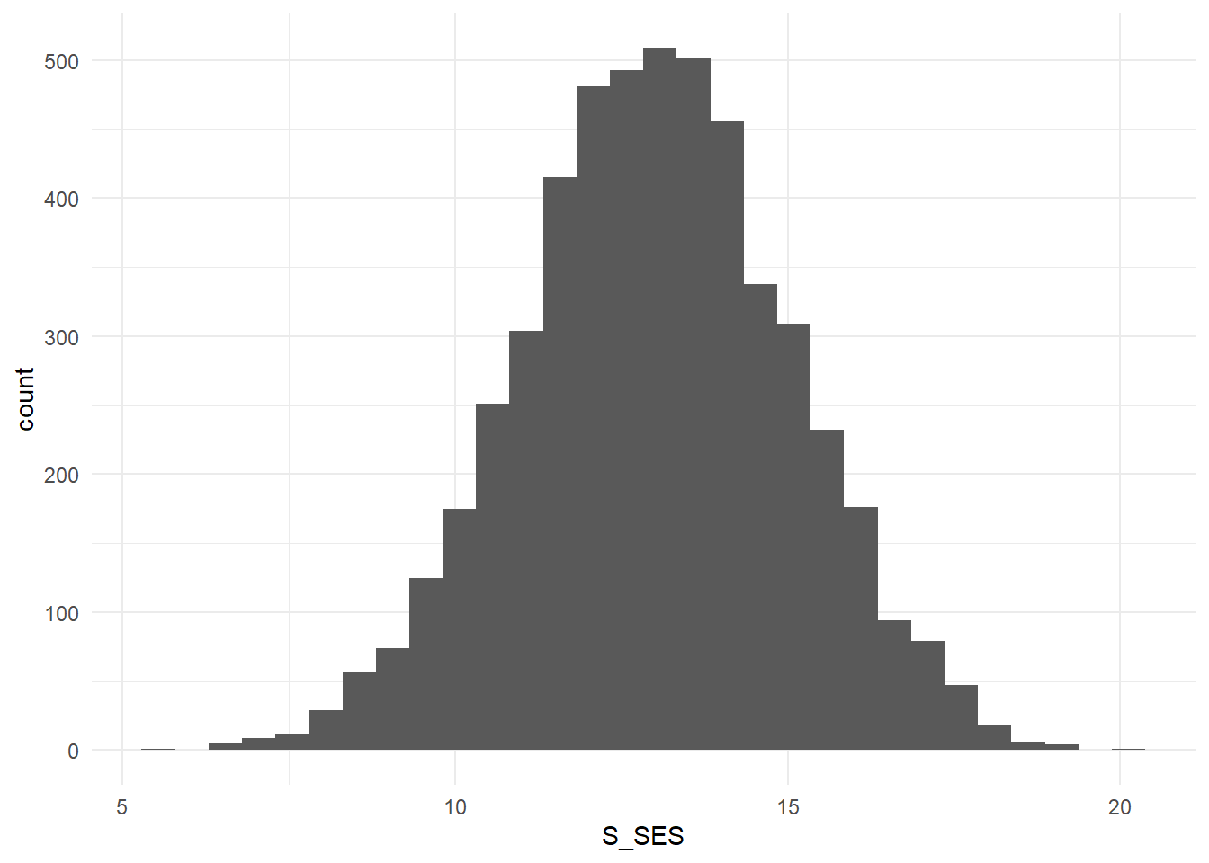
Figure 3.3: Distribution of Student SES
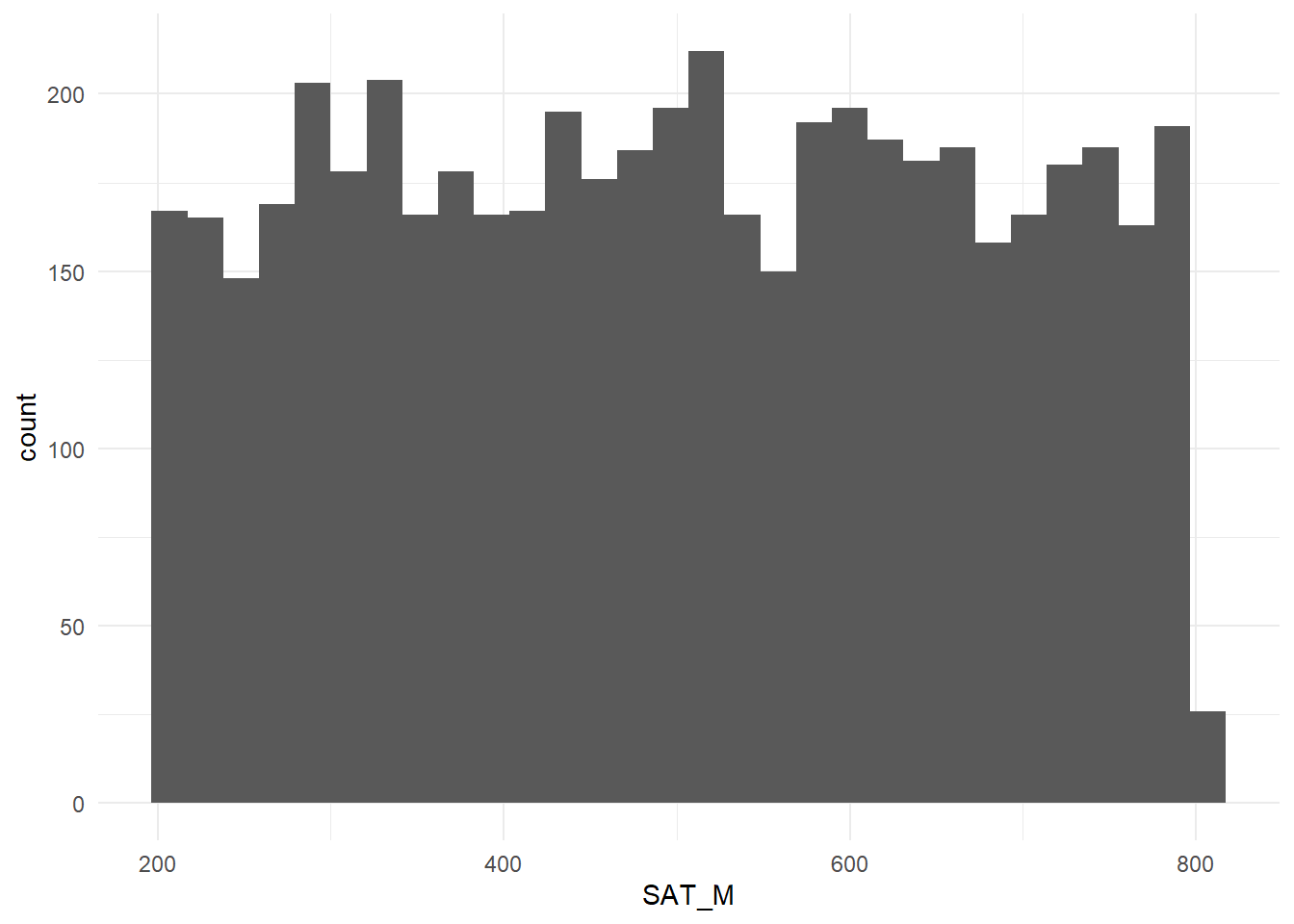
Figure 3.4: Distribution of Student SAT math scores
3.3 Software Considerations
MLwiN(Charlton et al., n.d.) is one of the most commonly found software programs for running multiple membership models, as it can natively handle such complex models. I have found that SAS and Stata can be ‘tricked’ into running simple multiple membership models by fitting them as constrained hierarchical models, but with non-continuous outcomes or increased complexity they quickly become computationally inefficient. More worrysome is that the parameter estimates generated by these methods are found to be biased. The same sources say that R can also be tricked (Leckie 2013a), as well as Bayesian estimation being possible by interfacing with JAGS software. Additionally, both R and Stata have functions or packages that allow you to use their interface and run MLwiN in the background, both to allow use of a familiar interface but also to allow for accurate estimation methods with full model recognition. MLwiN is not a free software and is produced by the University of Bristol. A 30-day free trial with full functionality is available to anyone in the world, and for researchers in the US, a single-user license is £400 or a PhD license is available for £225, though it expires after 3 years. In order to perform the analyses demonstrated below, I obtained a 30-day free license and used the R2MLwiN (Zhang et al. 2023) package to allow me to use an R interface. While the R code is provided, it will not work unless you also have a valid MLwiN license.
Heck, Reid, and Leckie (2022) used OpenBUGS for some more complex multiple membership cross classified modeling of longitudinal data, but at this time OpenBUGS website no longer exists and has been ported to MultiBUGS Goudie et al. (2020). One potential drawback of this program is the mis-classification of its software framework by virus detection programs as a virus, leading it to be uninstallable or to throw errors. MultiBUGS also reports that an R interface (R2MultiBUGS) is under development.