2 Data

The data set used for modelling can be found download from UC Irvine. The data set contains laboratory values of blood donors and Hepatitis C patients and demographic values like age. As mentioned, the focus is incorporating data science project and reports in an efficient format.

#Import Data

data<-read.csv("data/hcvdat0.csv",header = T,colClasses=c("NULL", rep(NA, 13))) 

#A quick summary - checking number of categorical and numeric variables
skimr::skim(data)[1:3]

Table 2.1: Data summary

Name	data
Number of rows	615
Number of columns	13
_______________________
Column type frequency:
character	2
numeric	11
________________________
Group variables	None

Variable type: character

skim_variable	n_missing
Category	0
Sex	0

Variable type: numeric

skim_variable	n_missing
Age	0
ALB	1
ALP	18
ALT	1
AST	0
BIL	0
CHE	0
CHOL	10
CREA	0
GGT	0
PROT	1

Modify the target variableCategoryinto binary so that Category= 0 if it falls into either”0=Blood Donor”or”0s=suspect Blood Donor”and 1 if it falls into any other categoryexcept being missing, in which case we keep it as is.

data$Category<-ifelse(data$Category=="0=Blood Donor" | data$Category=="0s=suspect Blood Donor",0,1)

#Frequency distribution of Category

table(data$Category)    

## 
##   0   1 
## 540  75

Frequency distribution shows “0”=570 and “1”=75.This shows an imbalanced classification problem since the frequency of response (Category) is skewed towards “0”. Observe Imbalanced classification problem. Methods for handling imbalanced classification problems such as undersampling and oversampling can be considered, however, that is beyond the scope or goal of this project.

2.1 Missing values and MICE Imputation.

colMeans(is.na(data))

##    Category         Age         Sex         ALB         ALP         ALT 
## 0.000000000 0.000000000 0.000000000 0.001626016 0.029268293 0.001626016 
##         AST         BIL         CHE        CHOL        CREA         GGT 
## 0.000000000 0.000000000 0.000000000 0.016260163 0.000000000 0.000000000 
##        PROT 
## 0.001626016

This shows the proportion of missing values in each column or varibale. We can observe that,ALP has the highest missing values.

#visualizing missing values
gg_miss_upset(data)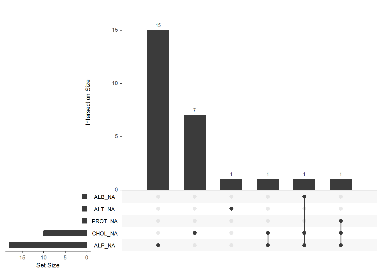

Mice Imputation for missing values.

#Model matric to tansform the data to numeric
data<-model.matrix(~.,data = data)
data<-data[,-1]