Introduction to dplyr

The dplyr library provides important functions through basic verbs that should make sense to use as we work with data. We will use the following functions to examine the iris dataset to answer some basic quantitative questions.

\(~\)

filter(), arrange(), select(), rename(), distinct(), mutate(), transmute(), summarise(), sample_n(), sample_frac()

\(~\)

First, maybe we would like to know just about one kind of iris, the iris setosa. First, we need to identify this within the data. Start by examining the help for the iris dataset in RStudio to figure out the exact syntax for the column containing species information. Now, we use this title to pass in the distinct() function, which will display the different values in the species column. Don’t forget to load the dplyr library before using these functions.

library(dplyr)

## 
## Attaching package: 'dplyr'

## The following objects are masked from 'package:stats':
## 
##     filter, lag

## The following objects are masked from 'package:base':
## 
##     intersect, setdiff, setequal, union

distinct(iris, Species)

##      Species
## 1     setosa
## 2 versicolor
## 3  virginica

\(~\)

We can create a new dataframe containing just the values from the setosa by using the select() function and naming the data setosa_df. Then we can display the top of the table with the kable() function, and create a simple histogram with the default plot from R.

setosa_df <- filter(iris, Species == "setosa")
kable(head(setosa_df))

Sepal.Length	Sepal.Width	Petal.Length	Petal.Width	Species
5.1	3.5	1.4	0.2	setosa
4.9	3.0	1.4	0.2	setosa
4.7	3.2	1.3	0.2	setosa
4.6	3.1	1.5	0.2	setosa
5.0	3.6	1.4	0.2	setosa
5.4	3.9	1.7	0.4	setosa

hist(setosa_df$Sepal.Length, main = "Histogram of Sepal Length of Iris Setosa", col = "beige", xlab = "Sepal Lengths")

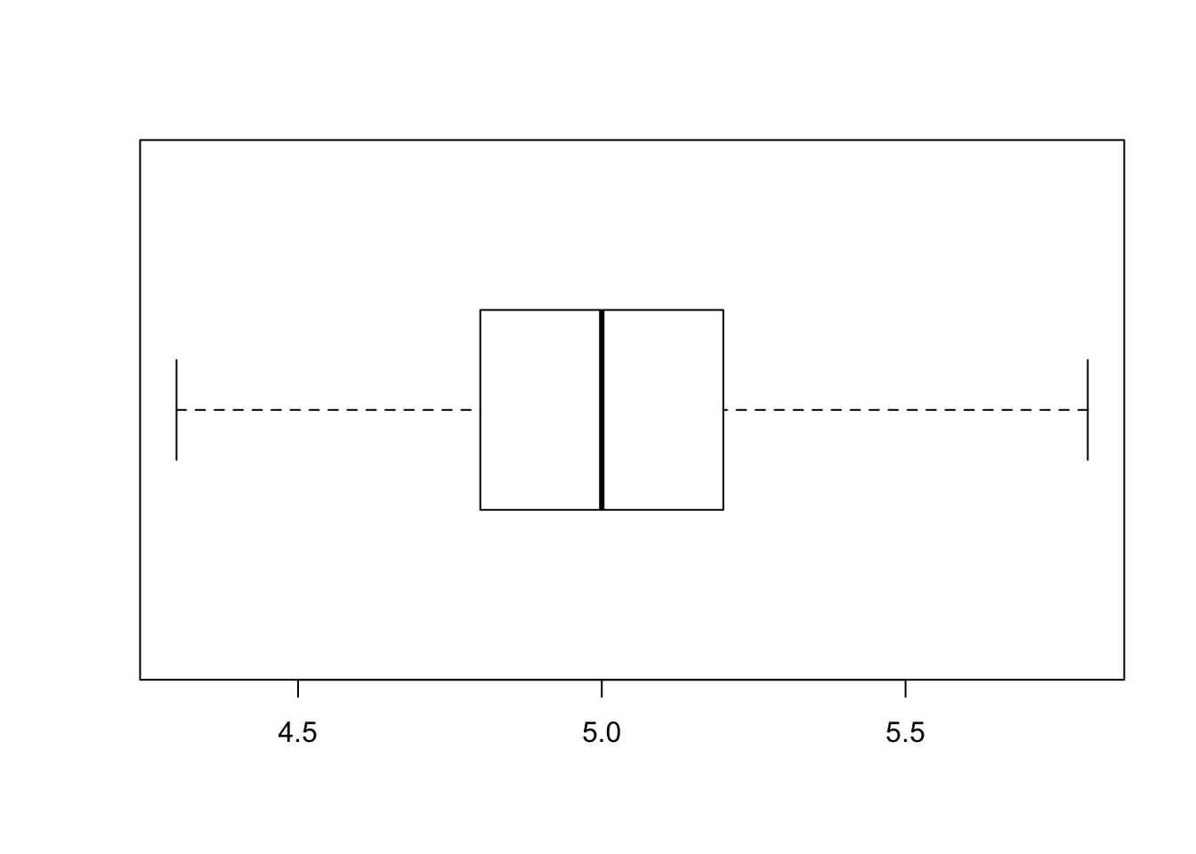
We can also get some quick descriptive statistical information about a dataframe with the summary() command. Further, we refer only to the first column of data here using setosa_df[, 1] to represent what we have plotted above. Finally, we can examine the data with a boxplot that is a typical visualization of the summary statistics.

summary(setosa_df[, 1])

##    Min. 1st Qu.  Median    Mean 3rd Qu.    Max. 
##   4.300   4.800   5.000   5.006   5.200   5.800

boxplot(setosa_df[, 1], horizontal = TRUE)