Analyzing the Lyrics

Now, we must consider the situation. Just because we have the text as individual words, this doesn’t mean we should assign equal importance to every word. There are many words stop words as we will refer to them, that do not need to be included. These include words like “to, the, of, …” you get the idea. There are preset stop words in the tidytext world, and we eliminate them by loading the stop_words and eliminating them with the anti_join() function as shown below. Further, we count and sort the lyrical content with count(word, sort = TRUE).

library(knitr)
data(stop_words)
tidy_ftp <- tidy_ftp %>%
              anti_join(stop_words) %>%
             count(word, sort = TRUE) 

## Joining, by = "word"

kable(head(tidy_ftp))

word	n
fight	18
power	14
hear	13
lemme	13
powers	5
people	3

Visualizing the Lyrics

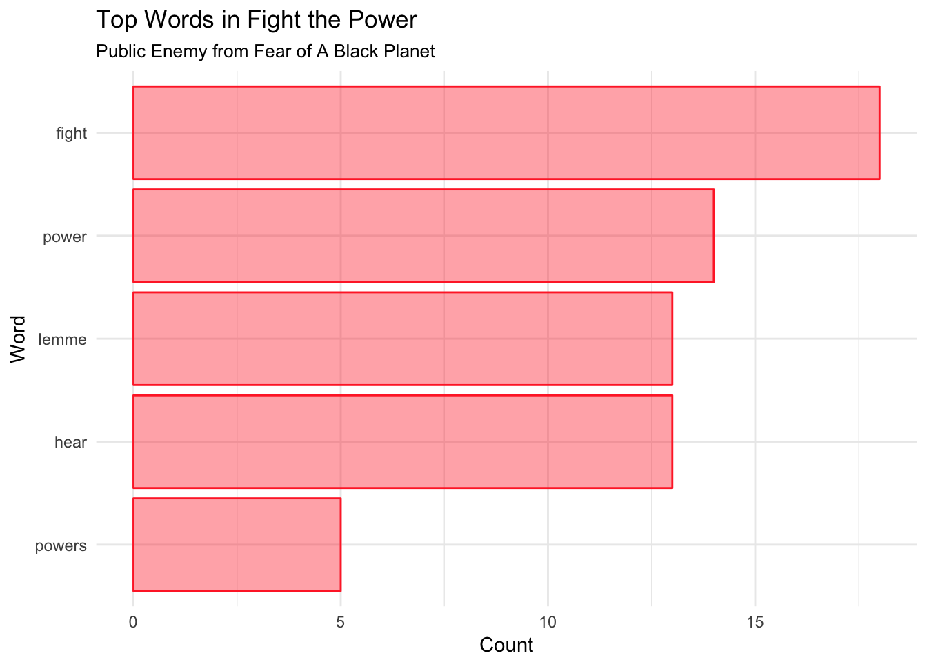
One question that we may ask is what are the top words used. From the previous table, we get a sense for the frequency of different words used. If we choose words that occur more than three times, this seems to be a good measure for top words here. We name the variable bars as the result of a pipe where we filter the words based on \(n > 3\) and reorder the column so that it is in decreasing order with the mutate function. We then display the table as a kable.

\(~\)

bars  <-  tidy_ftp %>%
            filter(n > 3) %>%
            mutate(word = reorder(word, n))

kable(head(bars))

word	n
fight	18
power	14
hear	13
lemme	13
powers	5

\(~\)

Now we can plot bars using ggplot.

\(~\)

ggplot(bars, aes(word, n)) +
    geom_col(stat = "identity", fill = "firebrick1",color = "firebrick1", alpha = 0.4) +
    labs(title = "Top Words in Fight the Power", subtitle = "Public Enemy from Fear of A Black Planet", x = "Word", y = "Count") +
    coord_flip() +
    theme_minimal()

## Warning: Ignoring unknown parameters: stat