Sec 1 Example of Time Series Data

library(astsa)

1.1 Characteristics of Time Series

1.1.1 Practical data

判斷以下範例為何不是 (weakly) stationary

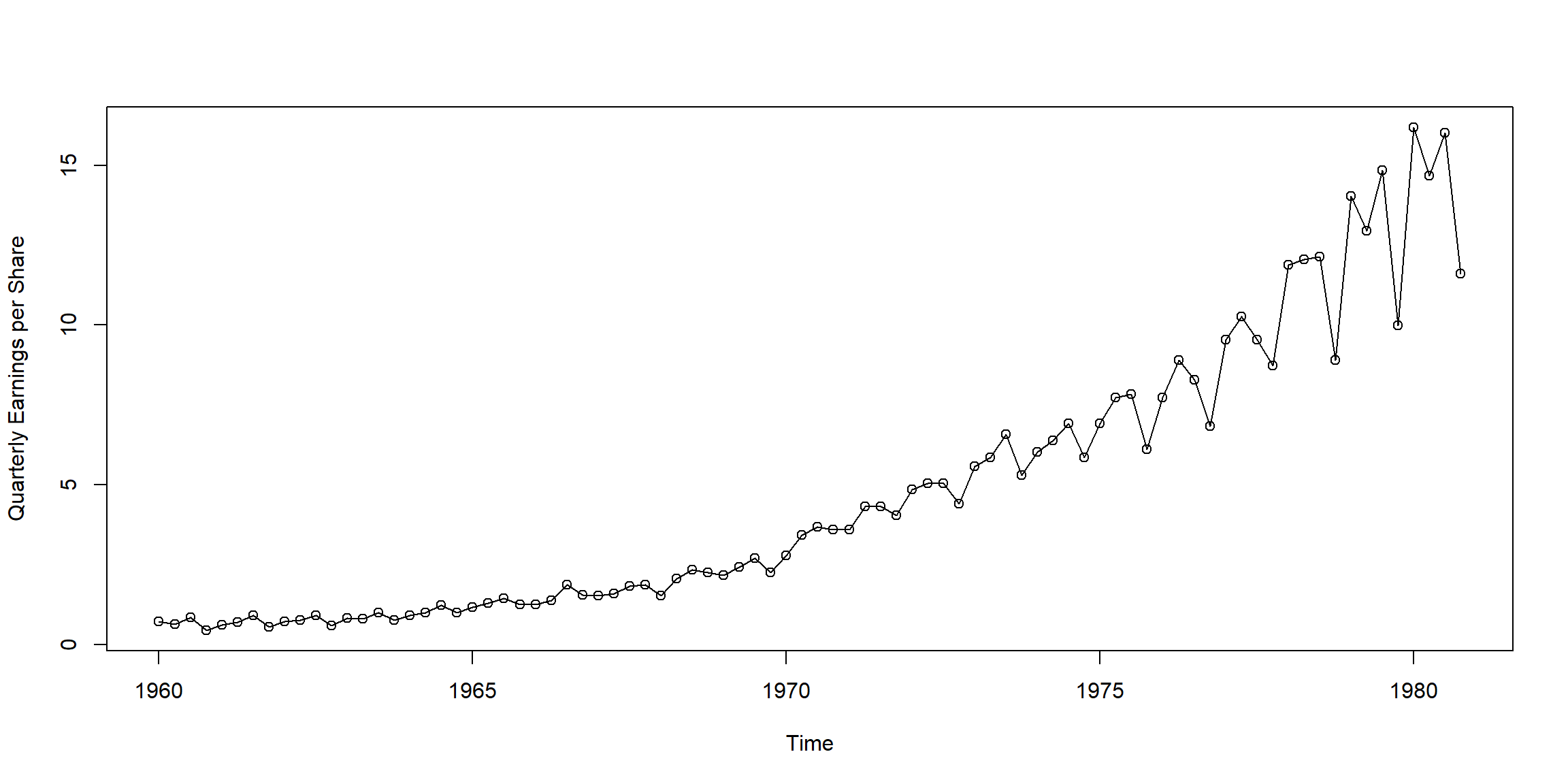
Example 1.1 (p.2)

plot(jj, type="o", ylab="Quarterly Earnings per Share")

trend
seasonality
heteroskedasticity

---

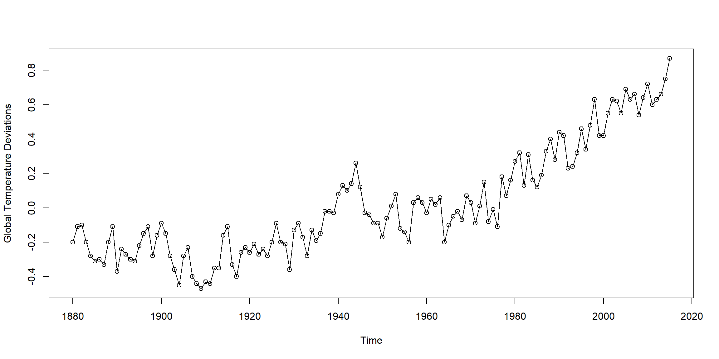
Example 1.2 (p.3)

plot(globtemp, type="o", ylab="Global Temperature Deviations")

trend
seasonality
heteroskedasticity

---

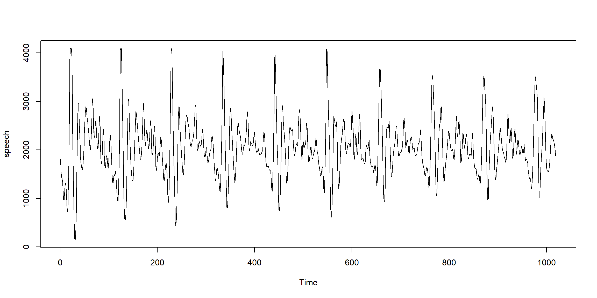
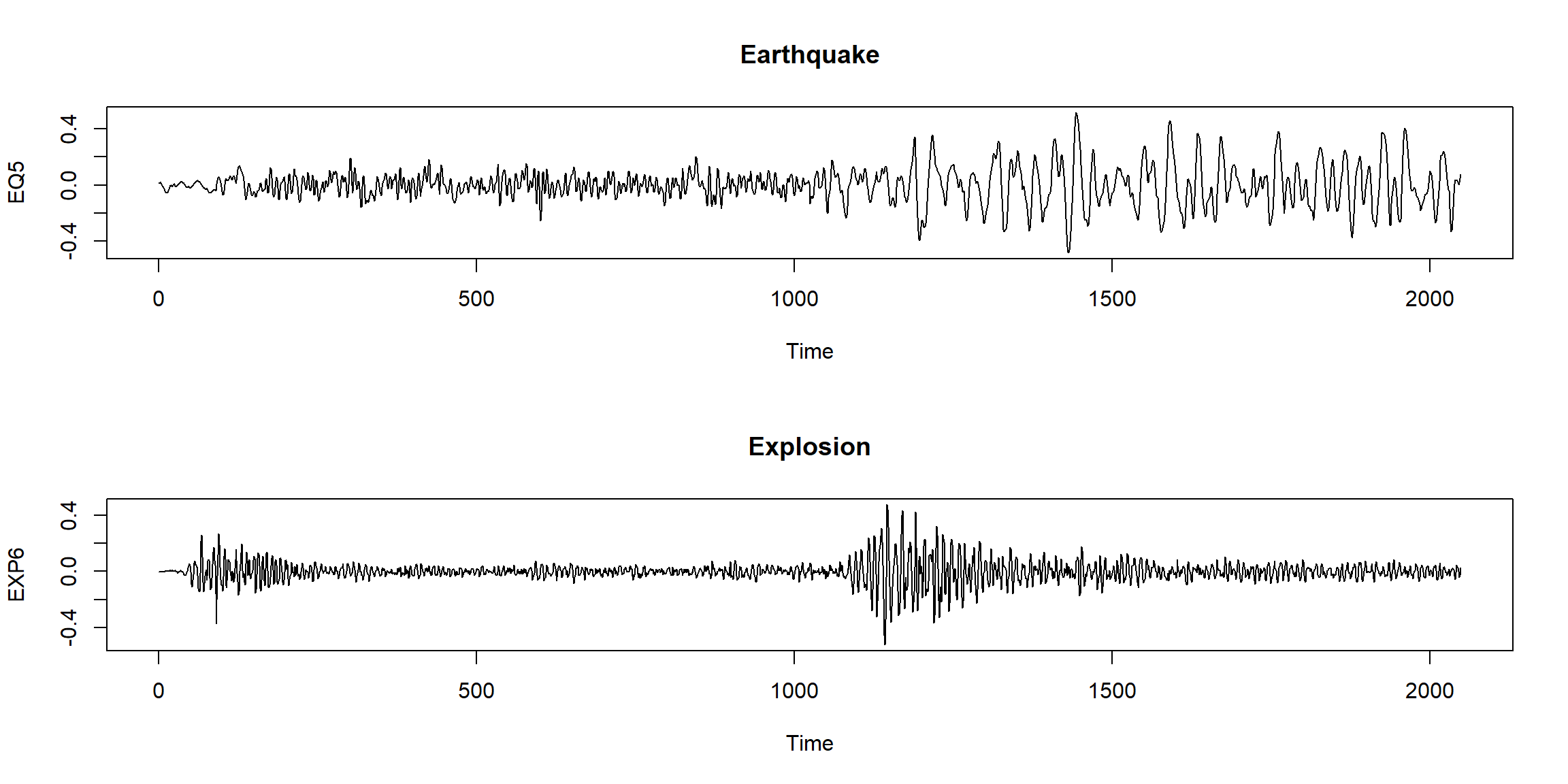
Example 1.3 (p.3) Voice record

plot(speech)

trend
seasonality
heteroskedasticity

---

Example 1.5 (p.5)

par(mfrow = c(2,1)) # set up the graphics
plot(soi, ylab="", xlab="", main="Southern Oscillation Index\nindex of ocean ccurrent 洋流")
plot(rec, ylab="", xlab="", main="Recruitment\nindex of fish amount")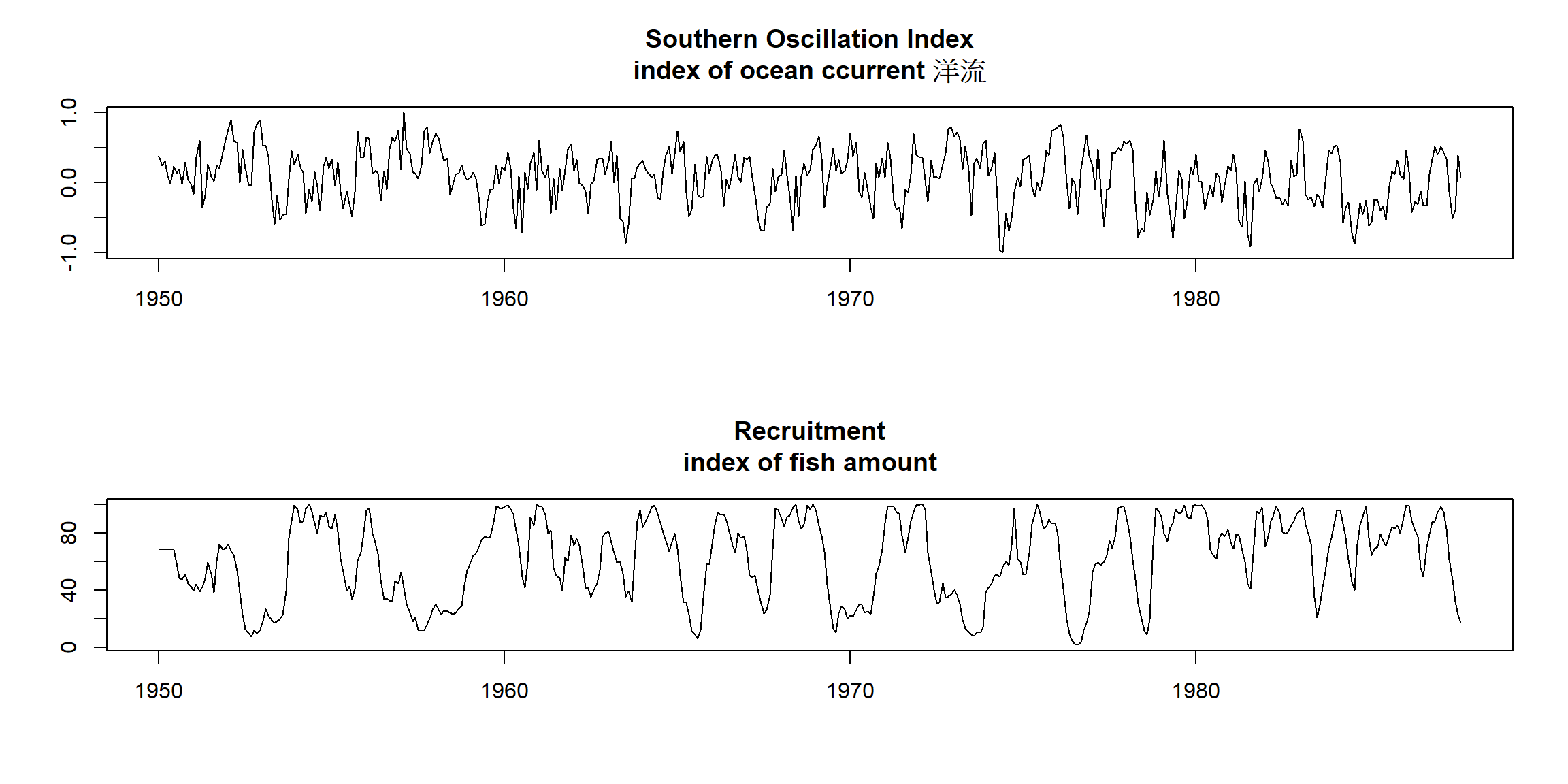

trend
seasonality
heteroskedasticity

---

Example 1.6 (p.5) MRI data

par(mfrow=c(2,1))
ts.plot(fmri1[,2:5], col=1:4, ylab="BOLD", main="Cortex")
ts.plot(fmri1[,6:9], col=1:4, ylab="BOLD", main="Thalamus & Cerebellum")
mtext("Time (1 pt = 2 sec)",side = 1,line = 2)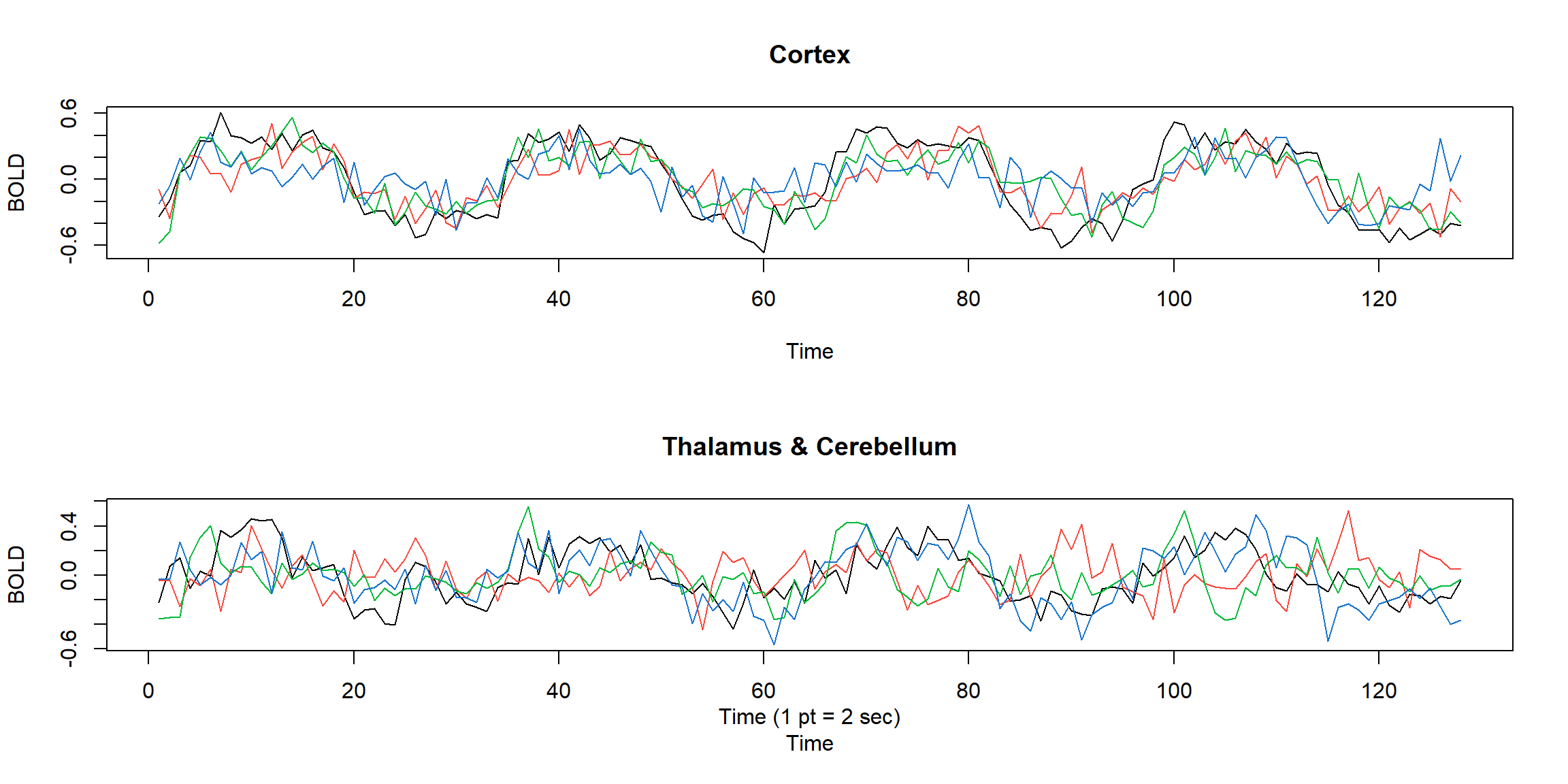

trend
seasonality
heteroskedasticity

---

Example 1.7 (p.6)

par(mfrow=c(2,1))
plot(EQ5, main="Earthquake")
plot(EXP6, main="Explosion")

trend
seasonality
heteroskedasticity

---

1.1.2 White Noise (WN)

Example 1.9 (p.10)

set.seed(0921)
w = rnorm(500,0,1) # 500 N(0,1) variates
v = filter(w, sides=2, filter=rep(1/3,3)) # moving average
par(mfrow=c(2,1))
plot.ts(w, main="white noise")
plot.ts(v, ylim=c(-3,3), main="moving average")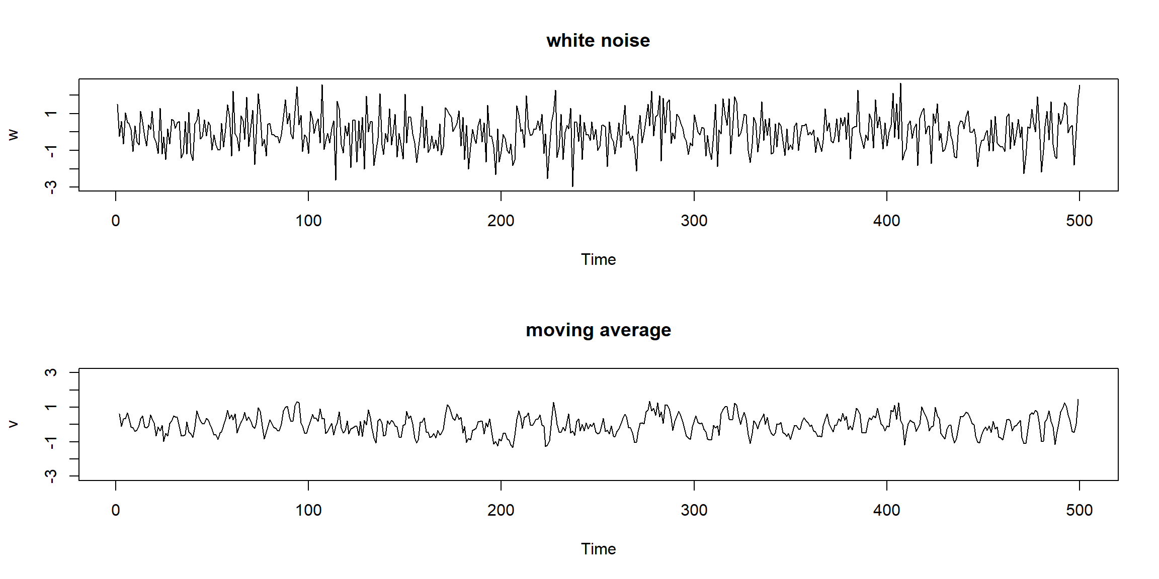

$$W_t\sim N(0,1)$$

• sides=2, center at lag 0

$$V_t=\frac1 3(W_{t-1}+W_t+W_{t+1})$$

• sides=1, for past value only

$$V_t=\frac1 3(W_t+W_{t-1}+W_{t-2})$$

---

Example 1.10 (p.11)

set.seed(0921)
w = rnorm(550,0,1) # 50 extra to avoid startup problems
x = filter(w, filter=c(1,-.9), method="recursive")[-(1:50)] # remove first 50
plot.ts(x, main="autoregression")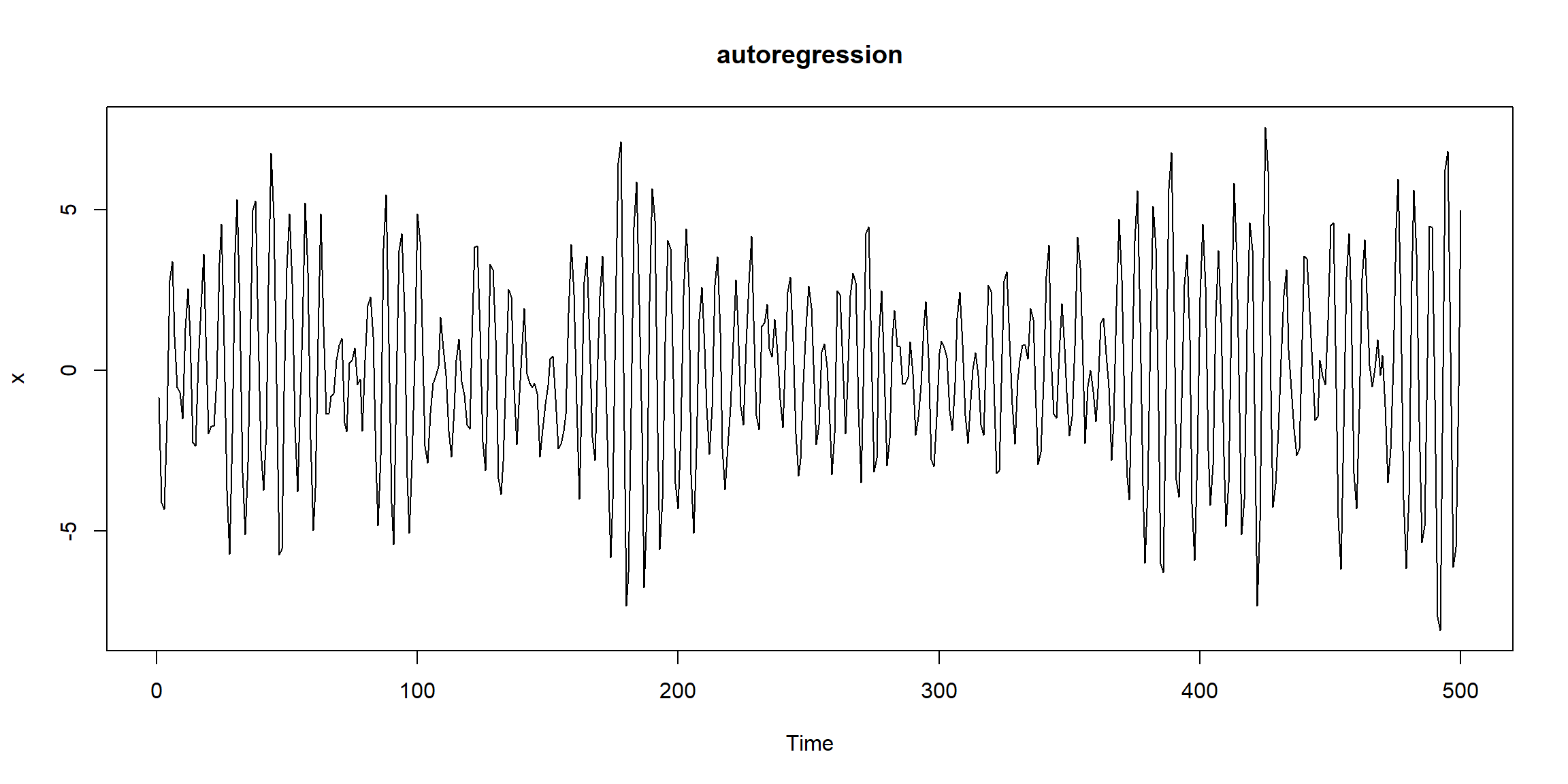

$$W_t\sim N(0,1)$$ $X_t=W_t-0.9W_{t-1}$ (default sides=1)

$X_t$ and $X_{t+1}$ are negatively correlated, means when

• $X_t\uparrow\:\Rightarrow X_{t+1}\downarrow$
  
• $X_t\downarrow\:\Rightarrow X_{t+1}\uparrow$
  

---

1.1.3 Random Walk

Example 1.11 (p.11)

set.seed(154) # so you can reproduce the results
w = rnorm(200,0,1); x = cumsum(w) # two commands in one line
wd = w +.2; xd = cumsum(wd)
plot.ts(xd, ylim=c(-5,55), main="random walk")
lines(x, col=2)
lines(.2*1:200,lty="dashed")
legend('topleft', col=c(1,2,1), lty=c(1,1,2), 
       legend = c(expression(X[d]),expression(X[t]),expression(E(X[t]))))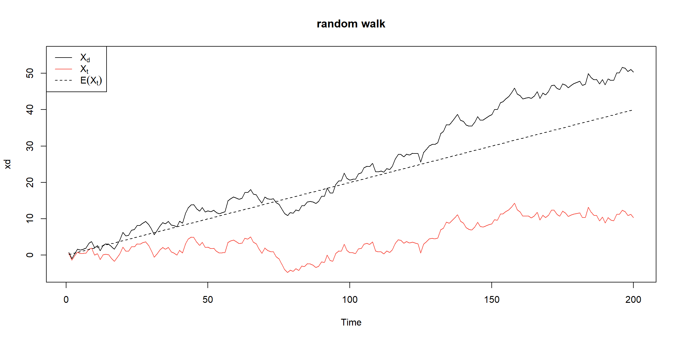

$X_t$ is not stationary, $\because Var(X_t)$ depends on t.

$X_d$ is not stationary, $\because E(X_d)$ depends on t.

• $W_t\sim N(0,1)$
• $X_t=W_1+W_2+...+W_t$
  • $Var(X_t)=Var(W_1)+Var(W_2)+...+Var(W_t)=1\cdot t=t$
• $W_d=W_t+0.2$
• $X_d=\sum W_d=\sum W_t+0.2\cdot t$
  • $E(X_d)=0.2\cdot t$

$E(aX+b)=aE(X)+b$
$Var(aX+b)=a^2Var(X)$

---

1.1.4 Noise influence periodic

Example 1.12 (p.12)

cs = 2*cos(2*pi*1:500/50 + .6*pi); w = rnorm(500,0,1)
par(mfrow=c(3,1), mar=c(3,2,2,1), cex.main=1.5)         # help(par) for info
plot.ts(cs, main=expression(x[t]==2*cos(2*pi*t/50+.6*pi)))
plot.ts(cs+w, main=expression(x[t]==2*cos(2*pi*t/50+.6*pi) + N(0,1)))
plot.ts(cs+5*w, main=expression(x[t]==2*cos(2*pi*t/50+.6*pi) + N(0,25)))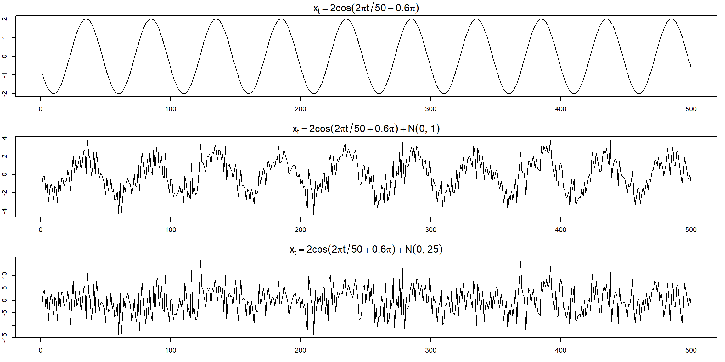

The periodic behavior became less obvious when the noise is large.

---

1.1.5 How lag influence plot

Example 1.24 (p.24) $$y_t=Ax_{t-l}+w_t$$

• $l>0$, $x_t$ lead $y_t$
  • $y_t=x_{t-1}+w_t$
  • $x$ lead $y$
• $l<0$, $x_t$ lag $y_t$
  • $y_t=x_{t+1}+w_t$
  • $x$ lag $y$

Assume $w_t$ is uncorrelated with $x_t$, the cross-covariance function is $$\gamma_{yx}(h)=cov(y_{t+h},x_t)=cov(Ax_{t+h-l}+w_{t+h},x_t)\\=cov(Ax_{t+h-l},x_t)=A\gamma_x(h-l)$$

When $h=l$, $\gamma_{yx}(h)=\gamma_x(0)$

x = rnorm(100)
y = lag(x, -5) + rnorm(100)
par(mfrow=c(1,1))
ccf <- ccf(y, x, type='covariance', 
           ylab='CCovF', xlab='lag h', main=expression(paste('l=5 with', hat(gamma)[yx](h))))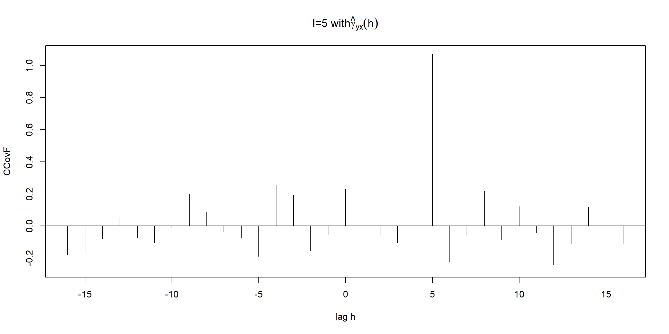

• $X\sim N(0,1)$
• $y_t=X_{t-5}+W_t, W_t\sim N(0,1)$
• $\require{enclose} \enclose{horizontalstrike}{Corr(y_t, X_{t+h})=\big\{\substack{1,\:h=5\\0,\:o.w.}}$
• $l=5\to\gamma_{yx}(h)=\gamma_x(h-5)$
  • $lag\:h=5 \to\gamma_{yx}(5)=\gamma_x(0)=variance(X)=1$
  • $y_{t+h}=Ax_{t+h-5}+w_{t+h}$
    • $i=|h-l|=|h-5|$
    • $h>5\to\gamma_{yx}(h)=cov(Ax_{t+i},x_t)\to x\:leads$
    • $h<5\to\gamma_{yx}(h)=cov(Ax_{t-i},x_t)\to y\:leads$

---

Example 1.25 (p.28)

par(mfrow=c(1,2))
r = round(acf(soi, 6, plot=FALSE)$acf[-1], 3)
plot(lag(soi,-1), soi, ylab=expression(X[t]), xlab=expression(X[t-1]))
arrows(-1,-1,1,1, col=2, angle = 15, lwd=5)
legend('topleft', legend=r[1])
plot(lag(soi,-6), soi, ylab=expression(X[t]), xlab=expression(X[t-6]))
arrows(-1,1,1,-1, col=2, angle = 15, lwd=5)
legend('topleft', legend=r[6])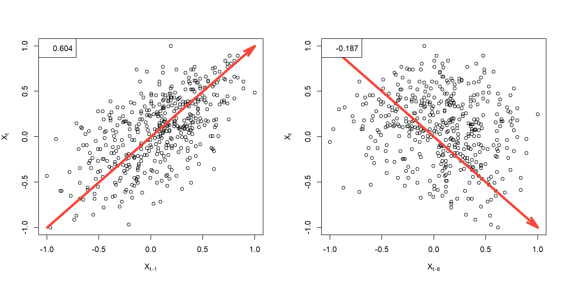

---

1.2 Explore Data

1.2.1 Estimate a linear trend

Example 2.1 (p.45) $$x_t=a+b\cdot t+W_t$$

summary(fit <- lm(chicken~time(chicken)))

## 
## Call:
## lm(formula = chicken ~ time(chicken))
## 
## Residuals:
##     Min      1Q  Median      3Q     Max 
## -8.7411 -3.4730  0.8251  2.7738 11.5804 
## 
## Coefficients:
##                 Estimate Std. Error t value Pr(>|t|)    
## (Intercept)   -7.131e+03  1.624e+02  -43.91   <2e-16 ***
## time(chicken)  3.592e+00  8.084e-02   44.43   <2e-16 ***
## ---
## Signif. codes:  0 '***' 0.001 '**' 0.01 '*' 0.05 '.' 0.1 ' ' 1
## 
## Residual standard error: 4.696 on 178 degrees of freedom
## Multiple R-squared:  0.9173, Adjusted R-squared:  0.9168 
## F-statistic:  1974 on 1 and 178 DF,  p-value: < 2.2e-16

plot(chicken, type="o",ylab="cents per pound")
abline(fit, lwd=2, col=2) # add regression line to the plot
legend('topleft', expression(a+bt), lwd=2, col=2)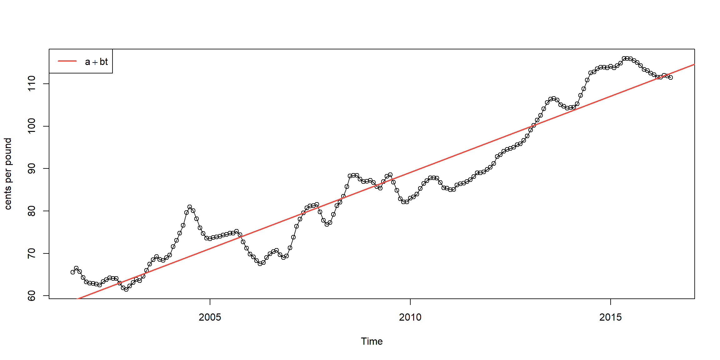

---

1.2.2 Detrend and Differencing

Example 2.4 and 2.5 (p.54, 58) $$x_t=a+b\cdot t+W_t$$

• detrended: $X_t-a-b\cdot t$
• first difference: $\nabla X_t=X_t-X_{t-1}$

fit = lm(chicken~time(chicken), na.action=NULL) # regress chicken on time
par(mfrow=c(2,1), mar=c(3,4,2,1))
plot(resid(fit), type="o", main="detrended")
plot(diff(chicken), type="o", main="first difference")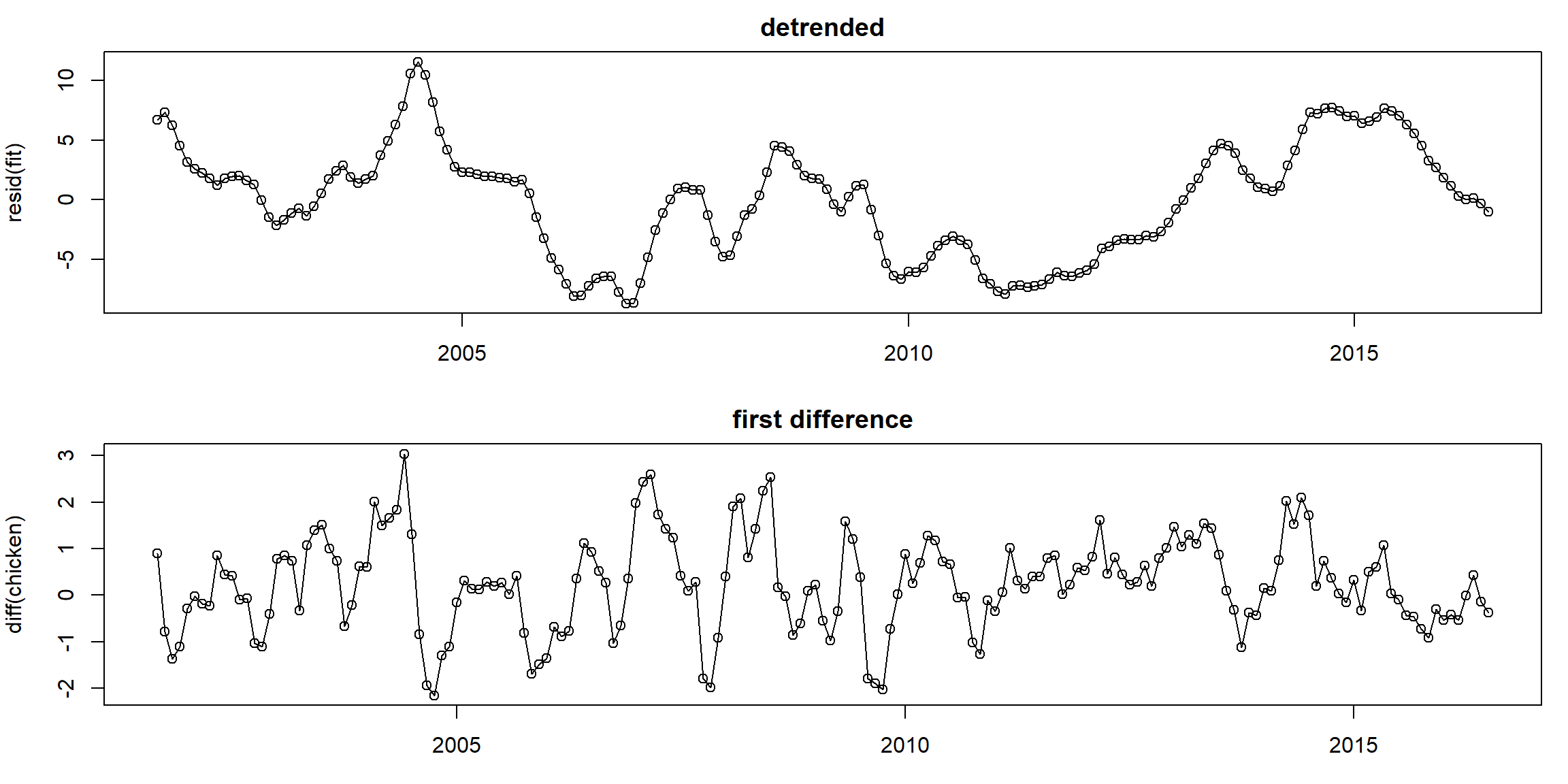

par(mfrow=c(3,1), mar=c(4,3,3,1)) # plot ACFs
acf(chicken, 48, main="chicken")
acf(resid(fit), 48, main="detrended")
acf(diff(chicken), 48, main="first difference")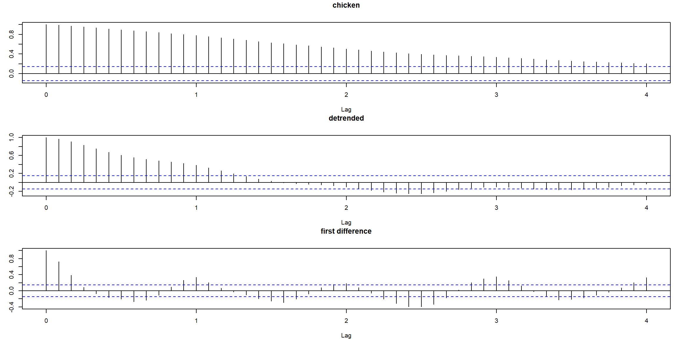

• first difference does better than regression
• ACF of stationary process decays fast to zero

---

Example 2.6 (p.58)

par(mfrow=c(2,1), mar=c(4,4,3,1))
plot(diff(globtemp), type="o")
mean(diff(globtemp)) # drift estimate = .008

## [1] 0.007925926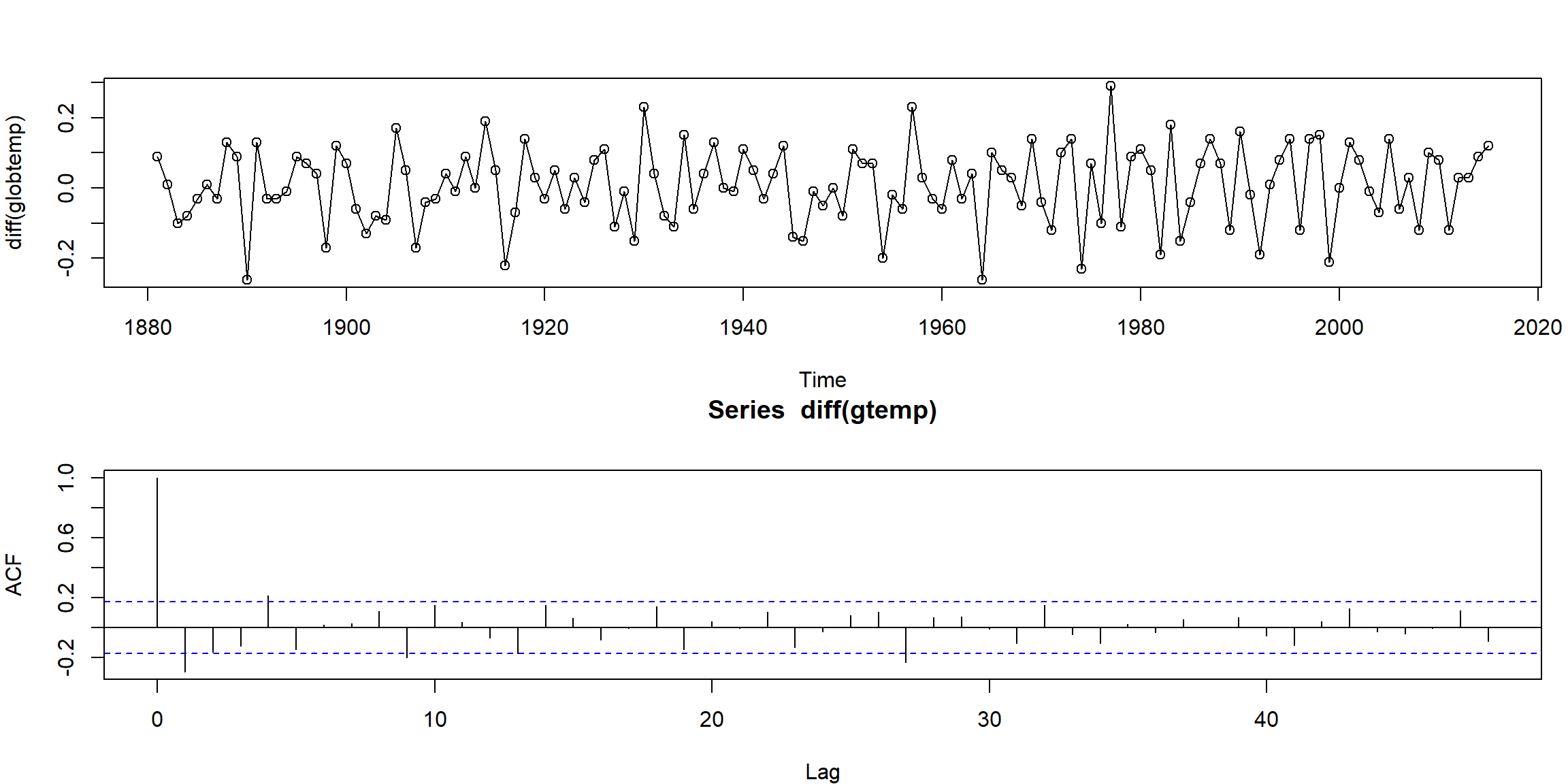

acf(diff(gtemp), 48)

• look stationary after first-order differencing

---

1.2.3 Smoothing

Example 2.13 (p.67) lowess

• lowess(x, y = NULL, f = 2/3)
  • f: the smoother span (band width)

plot(soi)
lines(lowess(soi, f=.05), lwd=2, col=4) # El Nino cycle
lines(lowess(soi), lty=2, lwd=2, col=2) # trend (with default span)
legend('topright', c('seasonality','trend'), col=c(4,2), lty=c(1,2), lwd=2)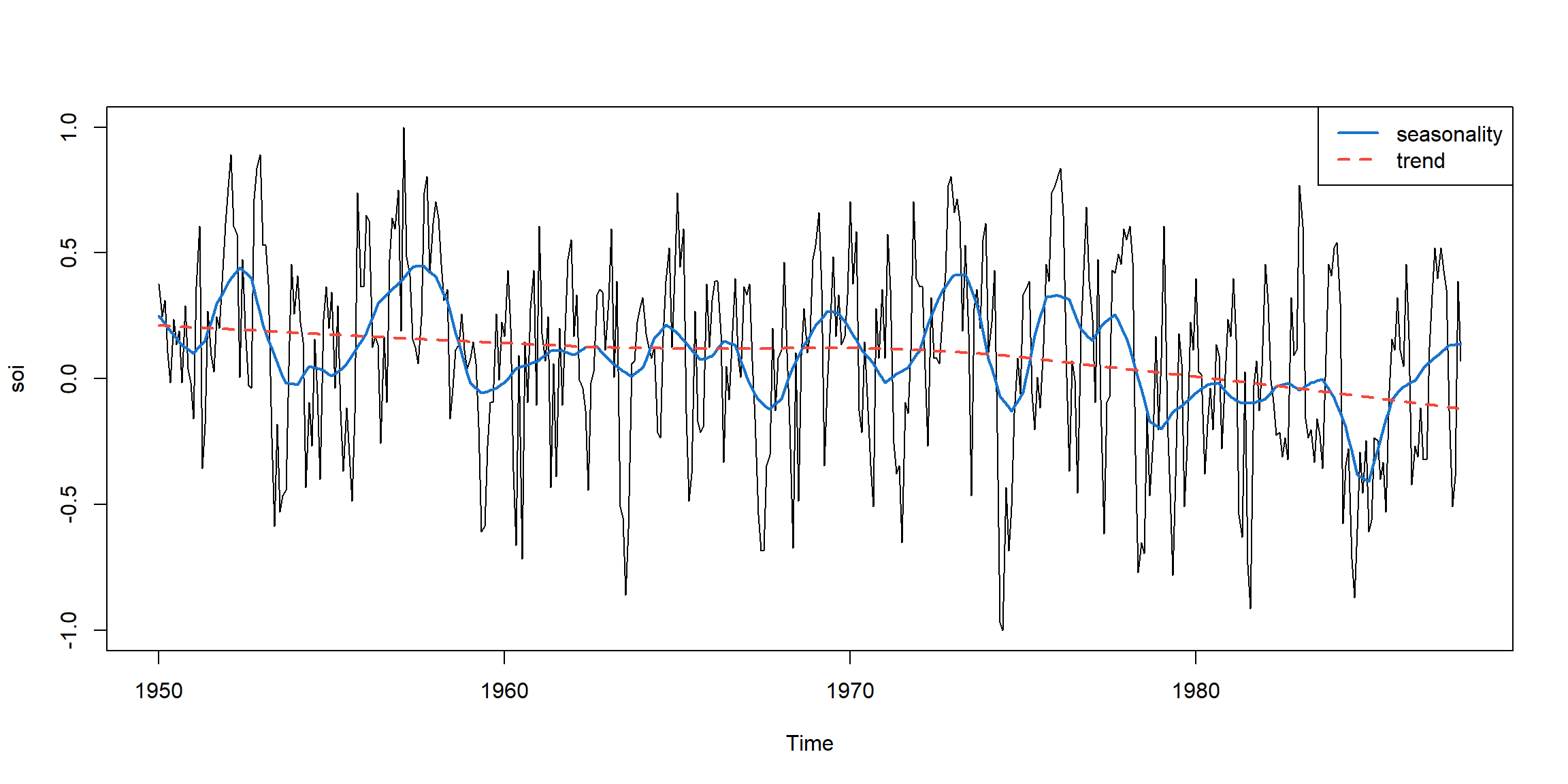

• seasonality: small band width
• trend: large band width

---

Example 2.14 (p.68) smooth.spline

• smooth.spline(x, y, spar = NULL)
  • x: predictor
  • y: response
  • spar: smoothing parameter, typically (but not necessarily) in (0,1]

plot(soi)
lines(smooth.spline(time(soi), soi, spar=.5), lwd=2, col=4)
lines(smooth.spline(time(soi), soi, spar= 1), lty=2, lwd=2, col=2)
legend('topright', c('seasonality','trend'), col=c(4,2), lty=c(1,2), lwd=2)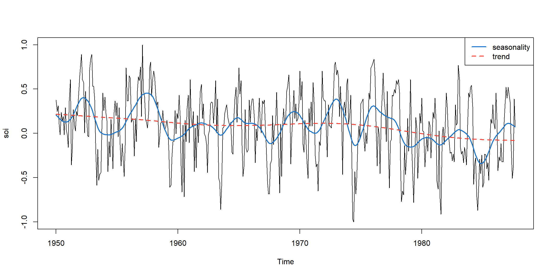

---

1.3 Time Series model

Example 3.2 (p.78) AR(1)

• arima.sim: Simulate from an ARIMA model.
  • order: c(p, d, q) $\to$ AR order, degree of differencing, MA order.
  • ARIMA(0,0,0) is white noise.
• If AR(2) $\to$ order=c(2,0,0), ar=c(.5, .1)

par(mfrow=c(2,1), mar=c(3,4,2,1))
plot(arima.sim(list(order=c(1,0,0), ar=.9), n=100), ylab="x",
     main=(expression(AR(1)~~~phi==+.9)))
plot(arima.sim(list(order=c(1,0,0), ar=-.9), n=100), ylab="x",
     main=(expression(AR(1)~~~phi==-.9)))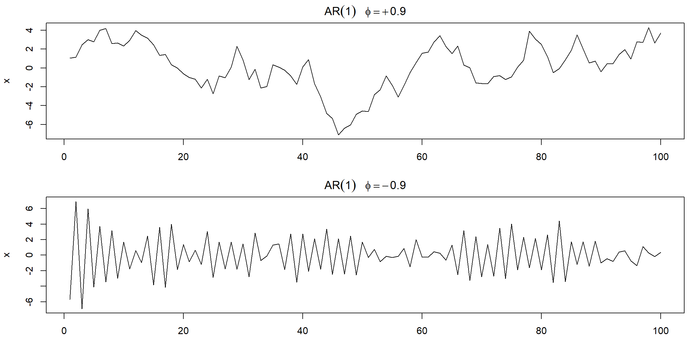

top	bottom
$\rho(h)=\color{red}{(0.9)}^h, h\geq0$	$\rho(h)=\color{red}{(-0.9)}^h, h\geq0$
positively correlated	negatively correlated
look like trend	fluctuate rapidly

---

Example 3.5 (p.82) MA MA(1) model $x_t=w_t+\theta w_{t-1}$ $$E(x_t)=0\\ \gamma(h)=\Bigg\{\begin{array}{ll} (1+\theta^2)\sigma^2_w,&h=0\\ \theta\sigma^2_w,&h=1\\ 0,&h>1 \end{array}\\ \rho(h)=\Big\{\begin{array}{ll} \frac{\theta}{1+\theta^2},&h=1\\ 0,&h>1 \end{array}$$

par(mfrow = c(2,1), mar=c(3,4,2,1))
plot(arima.sim(list(order=c(0,0,1), ma=.9), n=100), ylab="x",
     main=(expression(MA(1)~~~theta==+.5)))
plot(arima.sim(list(order=c(0,0,1), ma=-.9), n=100), ylab="x",
     main=(expression(MA(1)~~~theta==-.5)))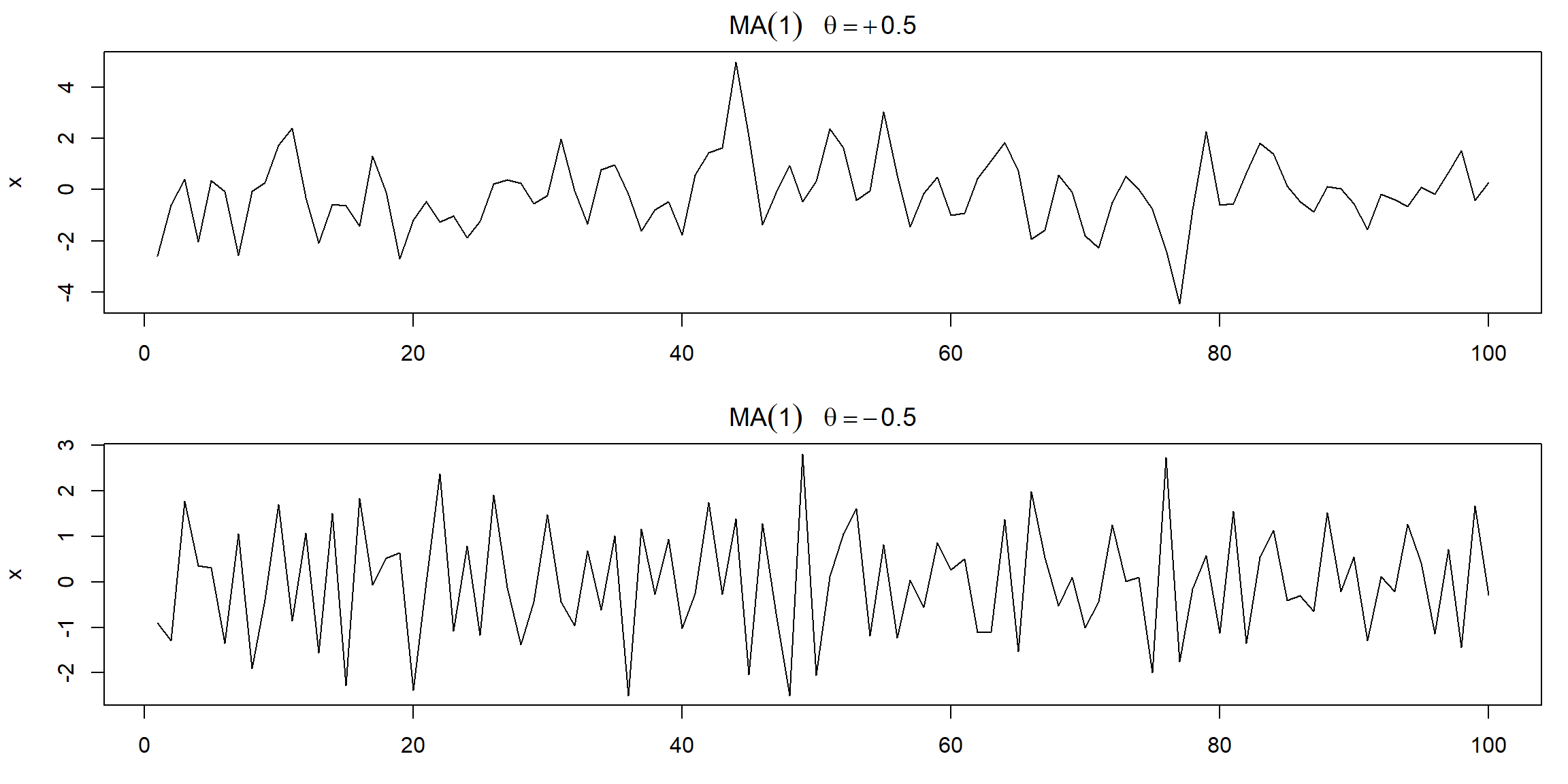

top	bottom
$\theta=0.5\Rightarrow x_t, x_{t-1}$ are positively correlated	$\theta=-0.5\Rightarrow x_t, x_{t-1}$ are negatively correlated
$\rho(1)=\frac{0.5}{1+0.5^2}=0.4\Rightarrow$ weak dependence

• The series for which $\theta=0.5$ is smoother than the series for $\theta=-0.5$.

---

Example 3.7 (p.84) parameter redundency If we were unaware of parameter redundancy, we might claim the data are correlated when in fact they are not

$$X_t\sim N(5,1),\text{ fit ARIMA(1,1) to X}\\ X_t=\phi X_{t-1}+W_t+\theta W_{t-1}$$

set.seed(8675309)
x = rnorm(150, mean=5) # generate iid N(5,1)s
out <- arima(x, order=c(1,0,1)); out # estimation

## 
## Call:
## arima(x = x, order = c(1, 0, 1))
## 
## Coefficients:
##           ar1     ma1  intercept
##       -0.9595  0.9527     5.0462
## s.e.   0.1688  0.1750     0.0727
## 
## sigma^2 estimated as 0.7986:  log likelihood = -195.98,  aic = 399.96

• $\phi=$ -0.96, $\theta=$ 0.95
• $(1+0.96B)X_t=(1+0.95B)W_t$

---

Example 3.8 (p.86) ARMA to MA

ARMAtoMA(ar = .9, ma = .5, 10) # for a list

##  [1] 1.4000000 1.2600000 1.1340000 1.0206000 0.9185400 0.8266860 0.7440174
##  [8] 0.6696157 0.6026541 0.5423887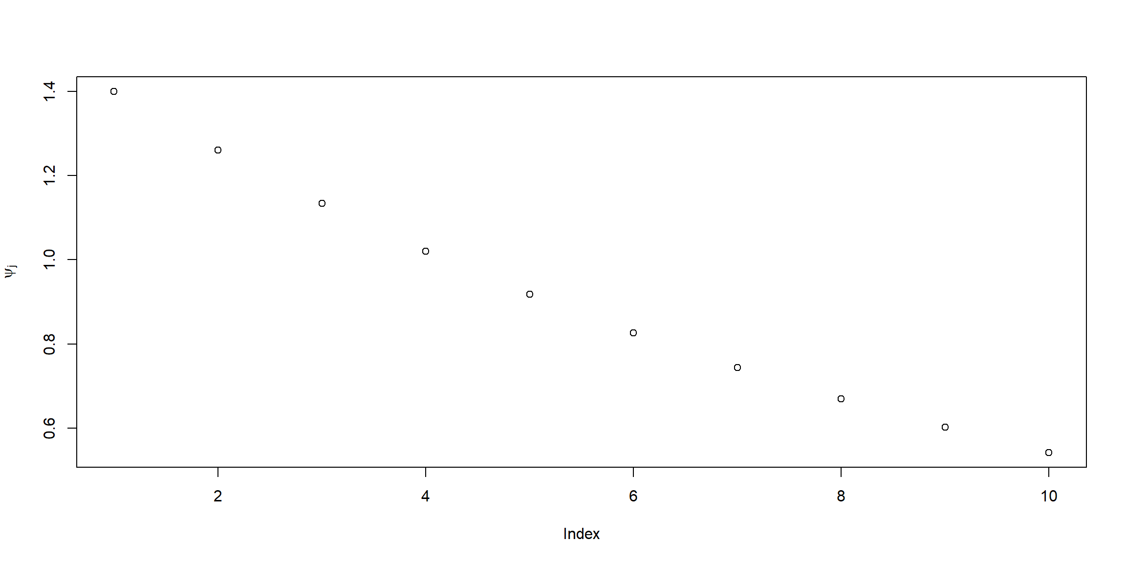

plot(ARMAtoMA(ar = .9, ma = .5, 10), 
     ylab = expression(psi [j]))

ARMAtoMA(ar = -.5, ma = -.9, 10) # first 10 pi-weights

##  [1] -1.400000000  0.700000000 -0.350000000  0.175000000 -0.087500000
##  [6]  0.043750000 -0.021875000  0.010937500 -0.005468750  0.002734375

---

Example 3.11 (p.92) AR(2)

z = c(1,-1.5,.75) # coefficients of the polynomial
(a = polyroot(z)[1]) # = 1+0.57735i,print one root = 1 + i/sqrt(3)

## [1] 1+0.57735i

• polyroot: 解根

$$f(x)=1-1.5x+0.75x^2$$

arg = Arg(a)/(2*pi) # arg in cycles/pt
1/arg # =12,the period

## [1] 12

$$z=x+iy\\ r=\sqrt{x^2+y^2}\\ \phi=Arg(z)\\ x=r\cdot cos(\phi),\;y=r\cdot sin(\phi)$$

set.seed(90210)
ar2 = arima.sim(list(order=c(2,0,0), ar=c(1.5,-.75)), n = 144)  # simulated data
plot(1:144/12,ar2,type="l",xlab="Time (one unit = 12 obs)")
abline(v=0:12, lty="dotted",lwd=2)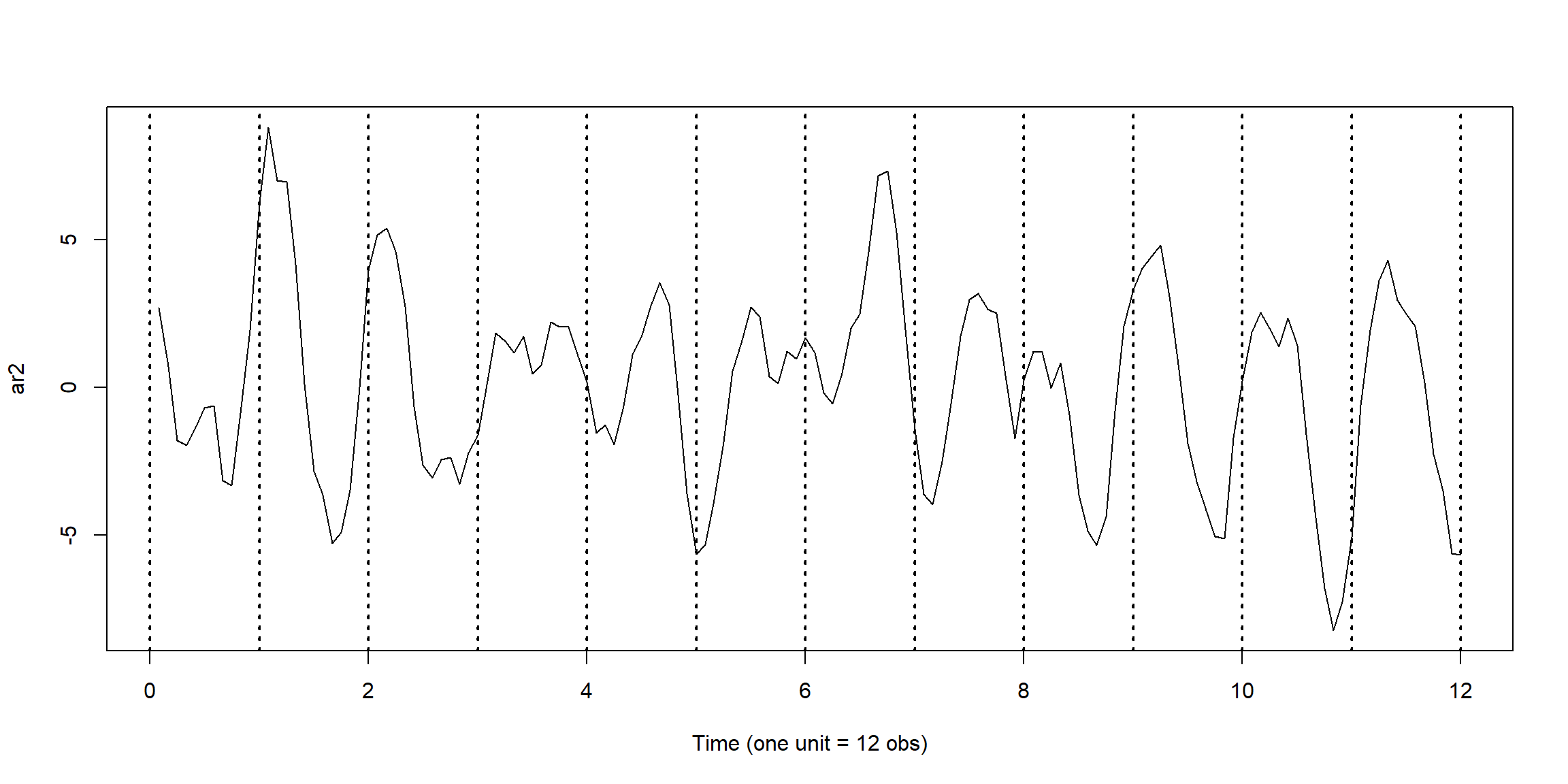

$$X_t=1.5X_{t-1}-0.75X_{t-2}+W_t$$

• has seasonality with period $d=12$
• AR(2) process is not stationary
• MA(q) process is always stationary

ACF = ARMAacf(ar=c(1.5,-.75), ma=0, 50) # theoretical
par(mfrow = c(2,1), mar=c(3,4,3,1))
plot(ACF, type="h", xlab="lag", main="theoretical ACF")
abline(h=0)
acf(ar2, lag.max = 50, main="sample ACF")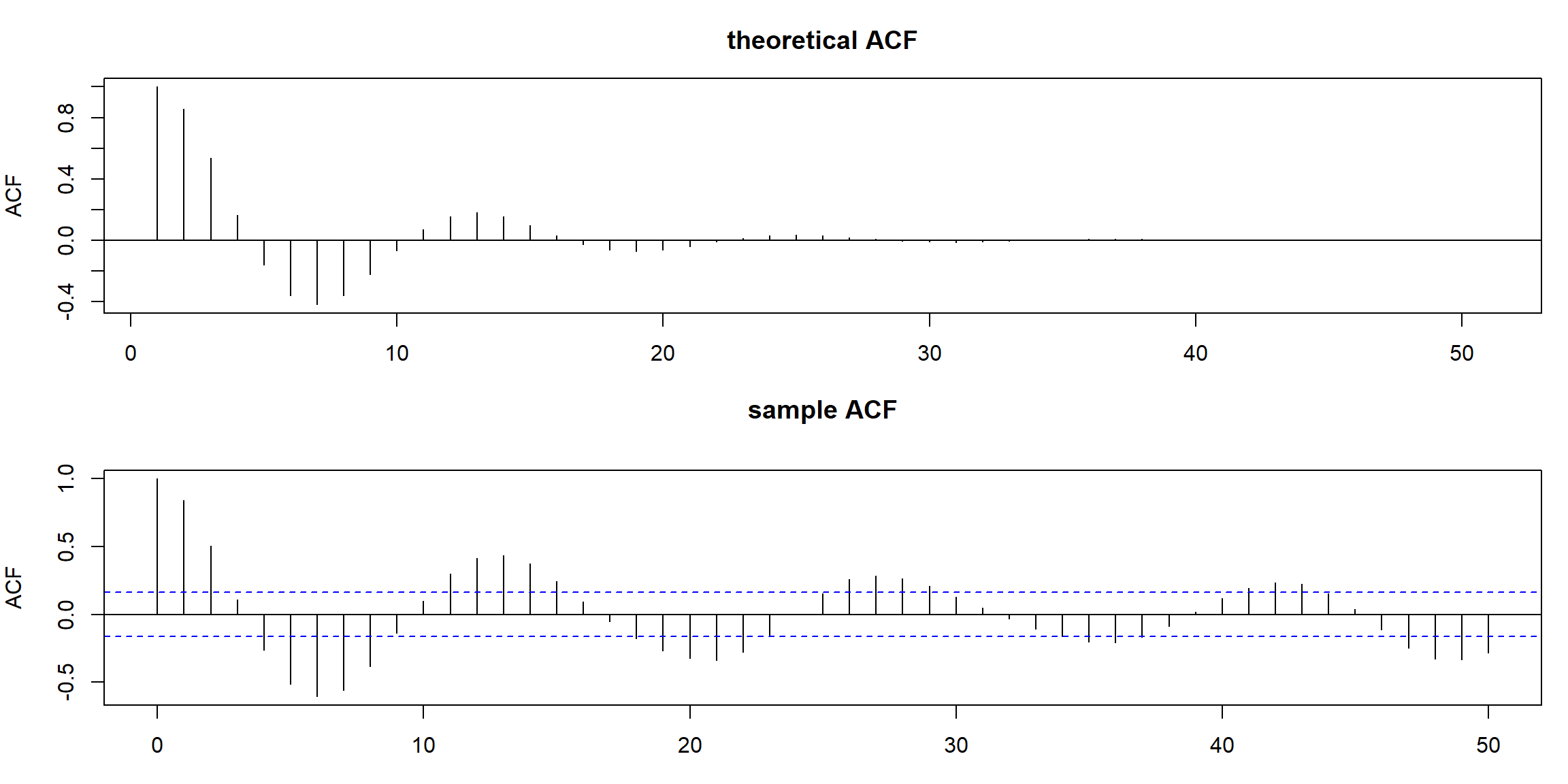

• ARMAacf: theoretical ACF (when model is given)
• acf: sample ACF (when data is given)
• ACF has periodic pattern

---

Example 3.16 (p.98) PACF of AR(p)

ar2.acf = ARMAacf(ar=c(1.5,-.75), ma=0, 24)[-1]
ar2.pacf = ARMAacf(ar=c(1.5,-.75), ma=0, 24, pacf=TRUE)
par(mfrow=c(1,2), mar=c(4,4,1,1))
plot(ar2.acf, type="h", xlab="lag"); abline(h=0)
plot(ar2.pacf, type="h", xlab="lag")
abline(h=0); axis(1, at=c(1:5))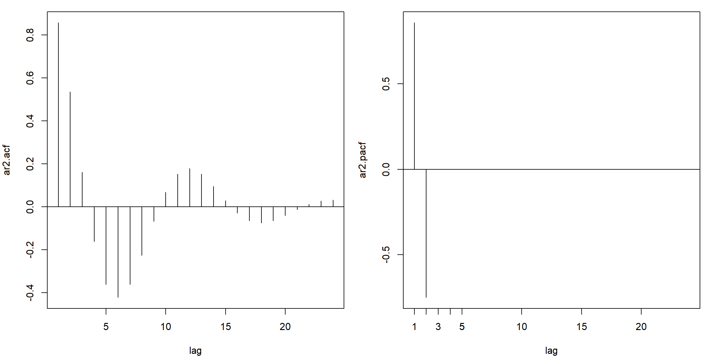

• PACF: cut off after lag 2

---

Example 3.29 (p.115) Simulate 50 obs. from MA(1) with $\theta_1=0.9$

set.seed(2)
ma1 = arima.sim(list(order = c(0,0,1), ma = 0.9), n = 50)
acf(ma1, plot=FALSE)[1] # = .507 (lag 1 sample ACF)

## 
## Autocorrelations of series 'ma1', by lag
## 
##     1 
## 0.507

• True ACF: $\rho(1)=\frac{\theta_1}{1+\theta_1^2}=$ 0.4972376

---

1.3.1 Behavior of the ACF and PACF for ARMA models

	AR(p)	MA(q)	ARMA(p, q)
ACF	Tails off	Cuts off after lag q	Tails off
PACF	Cuts off after lag p	Tails off	Tails off

1.4 Fit model with different method

在對資料進行建模前，可以用ACF, PACF初步分析，判斷p, q需要選多少

1.4.1 Preliminary Analysis

Example 3.18 (p.99) Preliminary Analysis of the Recruitment Series

value <- acf2(rec, 48) # will produce values and a graphic

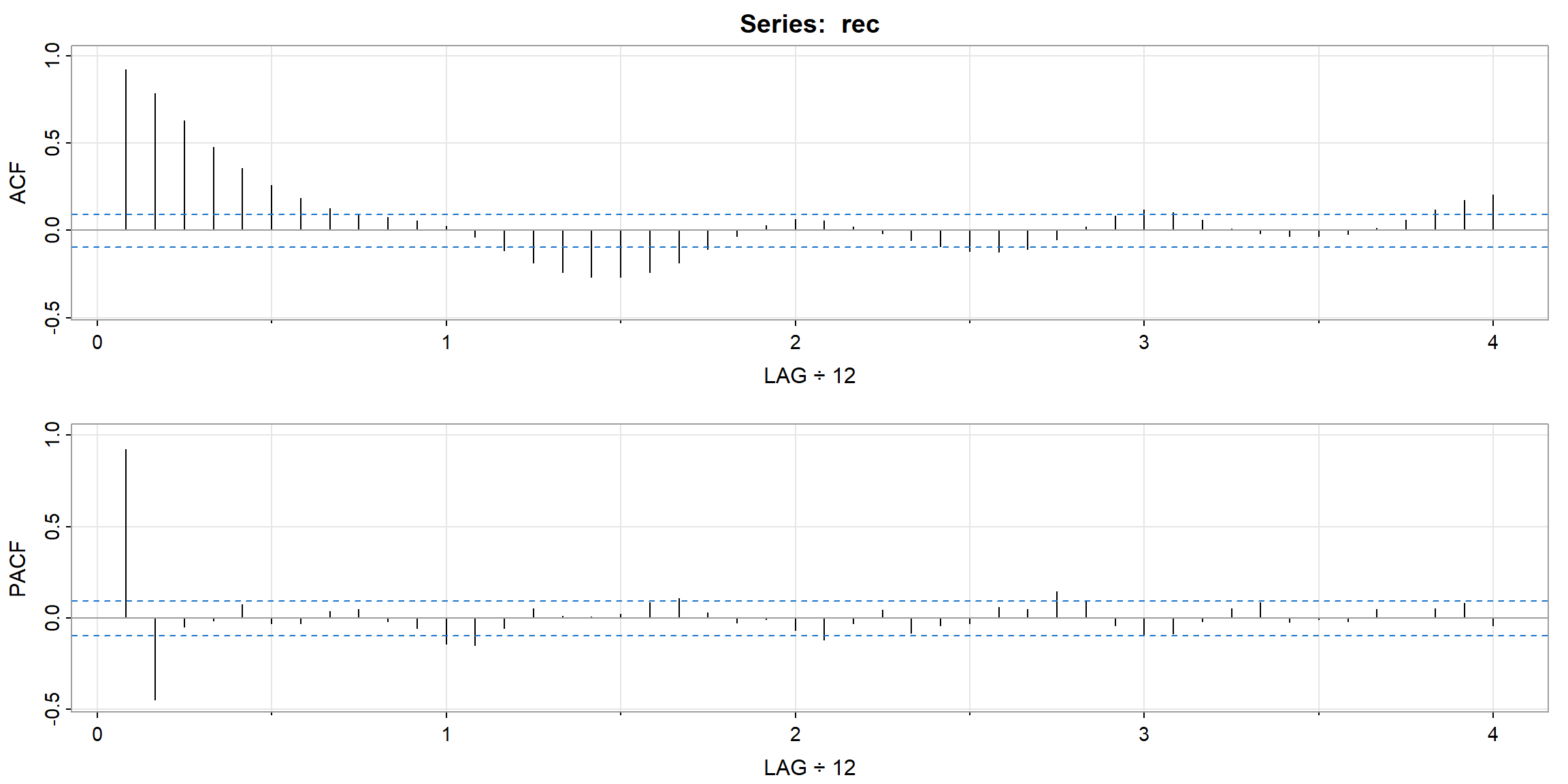
• ACF decay very fast $\to$ stationary
• PACF cut-off after lag 2 (its PACF $\approx$ 0 after lag 2) $\to$ AR(2) is suitable for the data

	1	2	3	4	5	6	7	8	9	10	11	12	13	14	15	16
ACF	0.92	0.78	0.63	0.48	0.36	0.26	0.18	0.13	0.09	0.07	0.06	0.02	-0.04	-0.12	-0.19	-0.24
PACF	0.92	-0.44	-0.05	-0.02	0.07	-0.03	-0.03	0.04	0.05	-0.02	-0.05	-0.14	-0.15	-0.05	0.05	0.01

	17	18	19	20	21	22	23	24	25	26	27	28	29	30	31	32
ACF	-0.27	-0.27	-0.24	-0.19	-0.11	-0.03	0.03	0.06	0.06	0.02	-0.02	-0.06	-0.09	-0.12	-0.13	-0.11
PACF	0.01	0.02	0.09	0.11	0.03	-0.03	-0.01	-0.07	-0.12	-0.03	0.05	-0.08	-0.04	-0.03	0.06	0.05

	33	34	35	36	37	38	39	40	41	42	43	44	45	46	47	48
ACF	-0.05	0.02	0.08	0.12	0.10	0.06	0.01	-0.02	-0.03	-0.03	-0.02	0.01	0.06	0.12	0.17	0.20
PACF	0.15	0.09	-0.04	-0.10	-0.09	-0.02	0.05	0.08	-0.02	-0.01	-0.02	0.05	0.01	0.05	0.08	-0.04

---

1.4.2 Fit AR(2) model to Recruitment Series

Example 3.25 (p.110) Fit AR(2) to rec data by OLS

regr = ar.ols(rec, order=2, demean=FALSE, intercept=TRUE)
fore = predict(regr, n.ahead=24)
ts.plot(rec, fore$pred, col=1:2, xlim=c(1980,1990), ylab="Recruitment")

# 95% CI
U = fore$pred+1.96*fore$se; L = fore$pred-1.96*fore$se
xx = c(time(U), rev(time(U))); yy = c(L, rev(U))
polygon(xx, yy, border = 8, col = gray(.6, alpha = .2))
lines(fore$pred, type="p", col=2)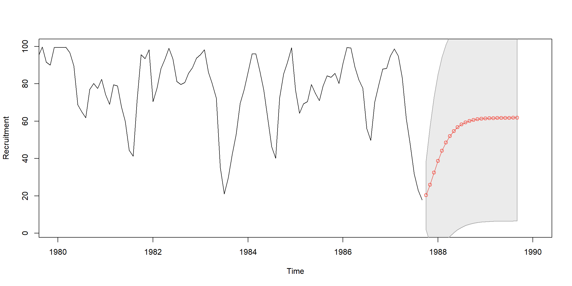

Example 3.28 (p.115) Fit AR(2) to rec data by Yule-Walker

rec.yw = ar.yw(rec, order=2)
rec.yw$x.mean # = 62.26278 (mean estimate)
rec.yw$ar # = 1.3315874, -.4445447 (coefficient estimates)
sqrt(diag(rec.yw$asy.var.coef)) # = .04222637, .04222637 (standard errors)
rec.yw$var.pred # = 94.79912 (error variance estimate)

rec.pr = predict(rec.yw, n.ahead=24)
# 95% CI
U=rec.pr$pred+1.96*rec.pr$se
L=rec.pr$pred-1.96*rec.pr$se
minx=min(rec,L);maxx=max(rec,U)
ts.plot(rec, rec.pr$pred, xlim=c(1980,1990),ylim=c(minx,maxx))
lines(rec.pr$pred,col="red",type="o")
lines(U, col="blue", lty="dashed")
lines(L, col="blue", lty="dashed")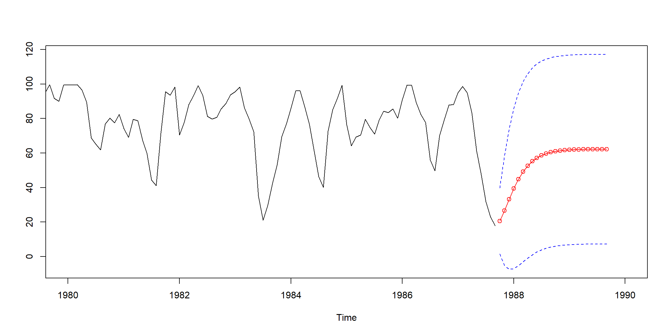

Example 3.31 (p.120) Fit AR(2) to rec data by MLE

rec.mle = ar.mle(rec, order=2)
rec.mle$x.mean # 62.26
rec.mle$ar # 1.35, -.46
sqrt(diag(rec.mle$asy.var.coef)) # .04, .04
rec.mle$var.pred # 89.34

1.4.3 compare AR(2) model’s coef. estimated by OLS, YW, and MLE

OLS	YW	MLE
1.354, -0.463	1.332, -0.445	1.351, -0.461

• Its coefficient estimator is similar

---

1.5 Analysis of GNP Data

Example 3.39, 3.40 (p.136, 139)

plot(gnp)

val <- acf2(gnp, 50)

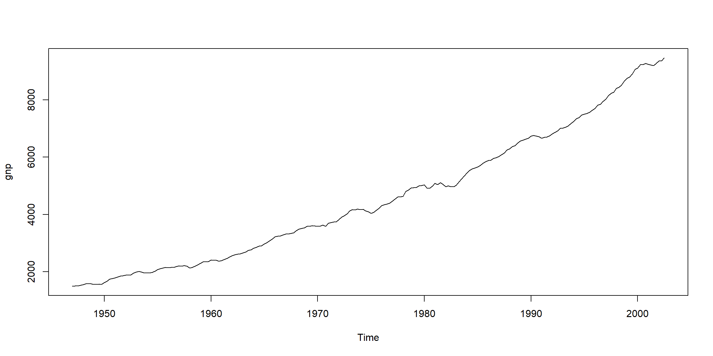
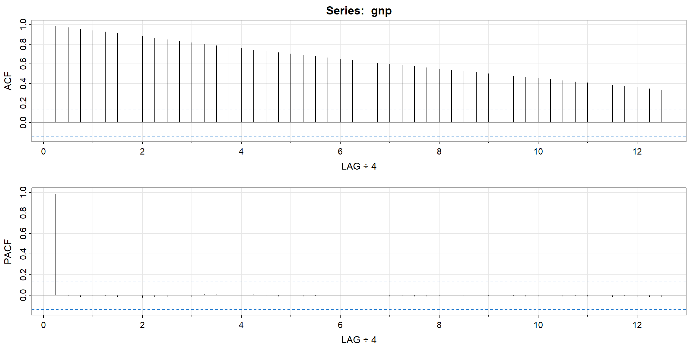
• ACF looks not stationary

gnpgr = diff(log(gnp)) # growth rate

• $diff(log(X_t))=logX_t-logX_{t-1}=log\frac{X_t}{X_{t-1}}, \;growth$
  • $diff(log(X_t))>0, \uparrow$
  • $diff(log(X_t))<0, \downarrow$

plot(gnpgr, ylab="GNP growth rate", lwd=2)
abline(h=mean(gnpgr), lty=2, col=2, lwd=2)
legend("topright", legend = "average growth rate", lty=2, lwd=2, col=2)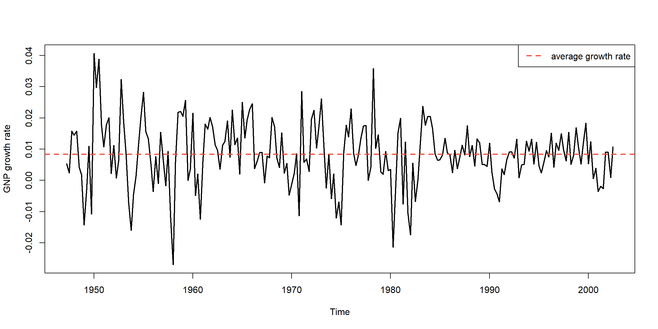

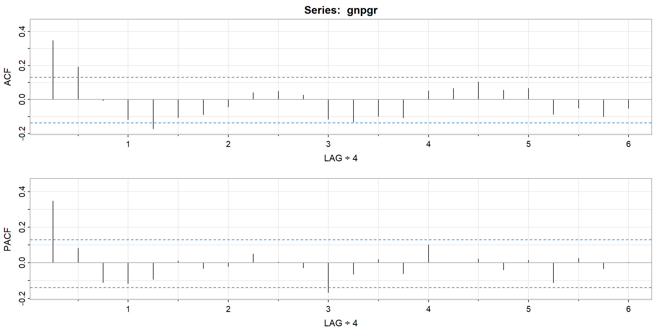
val <- acf2(gnpgr, 24)

• ACF cut-off after lag 2 $\Rightarrow$ MA(2)
• PACF cut-off after lag 1 $\Rightarrow$ AR(1)

	1	2	3	4	5	6	7	8	9	10	11	12
ACF	0.35	0.19	-0.01	-0.12	-0.17	-0.11	-0.09	-0.04	0.04	0.05	0.03	-0.12
PACF	0.35	0.08	-0.11	-0.12	-0.09	0.01	-0.03	-0.02	0.05	0.01	-0.03	-0.17

	13	14	15	16	17	18	19	20	21	22	23	24
ACF	-0.13	-0.10	-0.11	0.05	0.07	0.10	0.06	0.07	-0.09	-0.05	-0.10	-0.05
PACF	-0.06	0.02	-0.06	0.10	0.00	0.02	-0.04	0.01	-0.11	0.03	-0.03	0.00

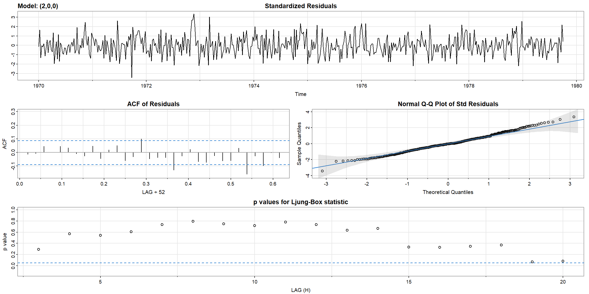
1.5.1 Diagnostics

out1 <- sarima(gnpgr, 1, 0, 0) # AR(1)

out2 <- sarima(gnpgr, 0, 0, 2) # MA(2)

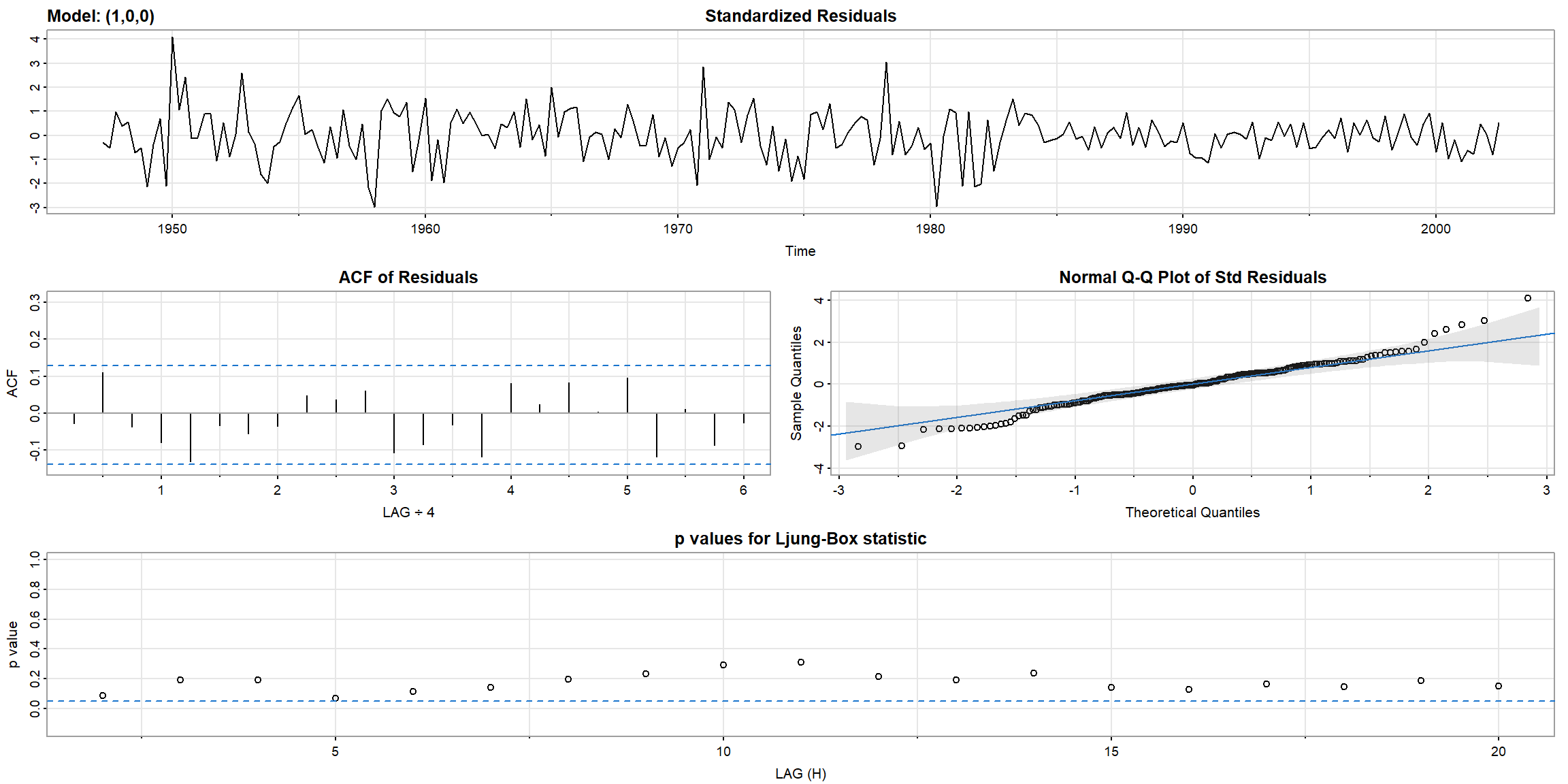
• In Ljung-Box statistic, both model’s p-value>0.05, $\therefore$ AR(1) is suitable for gnpgr

ARMAtoMA(ar=.35, ma=0, 10) # prints psi-weights

##  [1] 3.500000e-01 1.225000e-01 4.287500e-02 1.500625e-02 5.252187e-03
##  [6] 1.838266e-03 6.433930e-04 2.251875e-04 7.881564e-05 2.758547e-05

1.5.2 model selection

Both AR(1) and MA(2) are suitable. Then, which one is better?

• Use AIC, AICC or BIC, the smaller the better.

model	AIC	AICc	BIC
AR(1)	-6.44694	-6.4466932	-6.4009579
MA(2)	-6.4501328	-6.4496369	-6.3888233

• Since MA(2) model’s AIC, AICC and BIC are smaller than AR(1) model’s, MA(2) is better.

---

1.6 Model Diagnostics

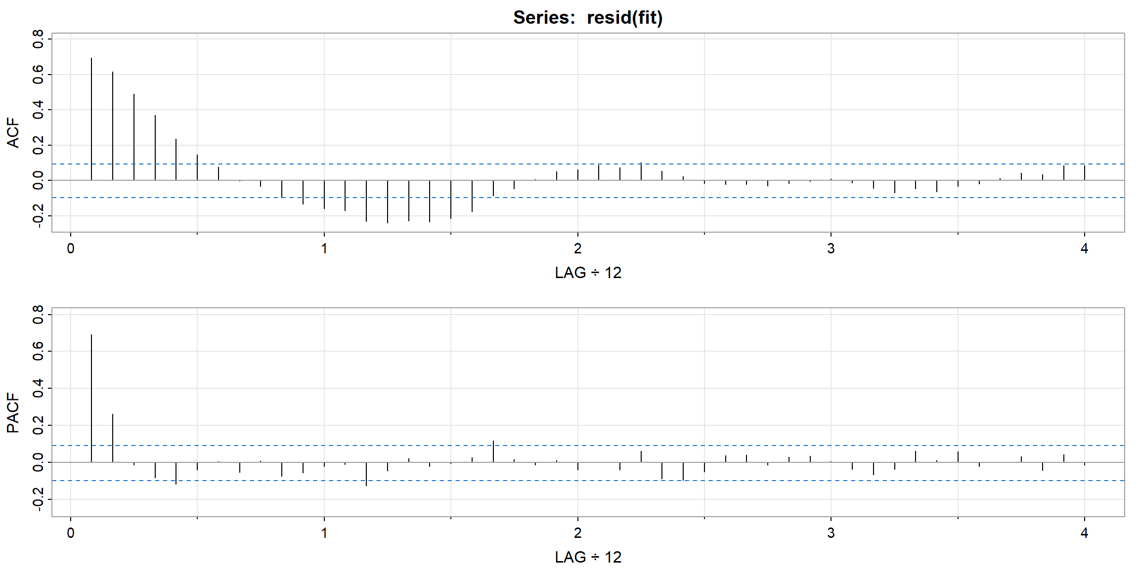
Example 3.41 (p.140) Diagnostics for the Glacial Varve Series

sarima(log(varve), 0, 1, 1, no.constant=TRUE) # ARIMA(0,1,1)

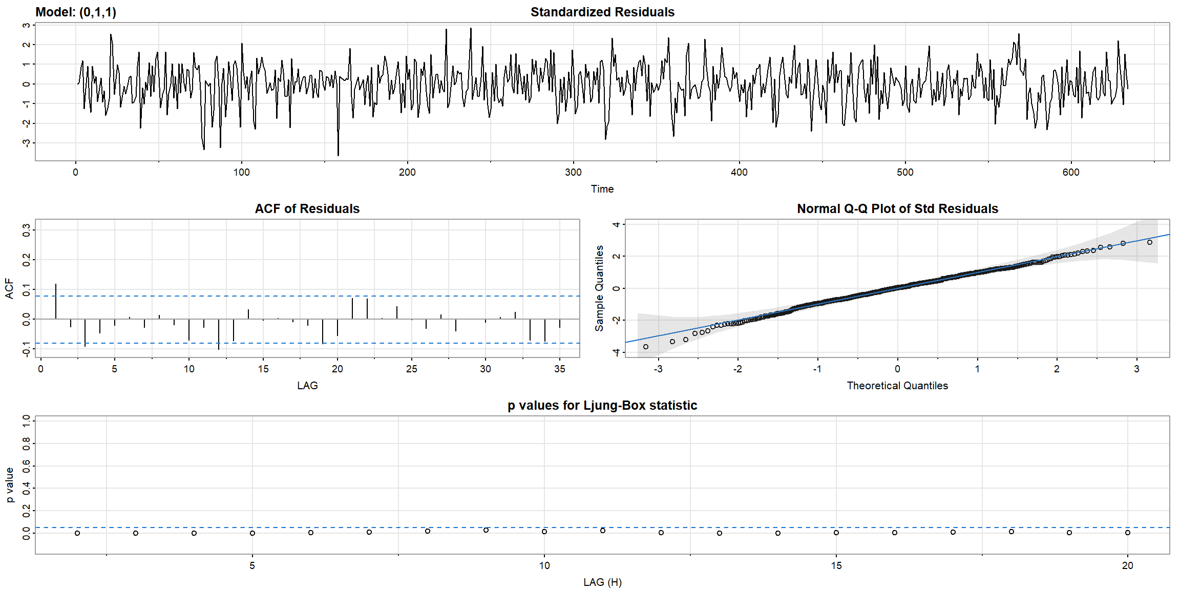
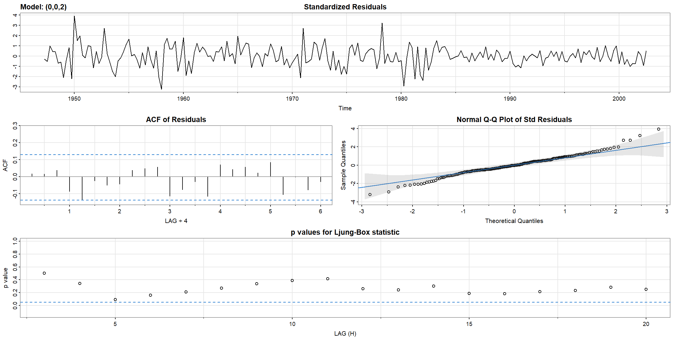
• ACF outside the CI, and p-value$$0.05, $\therefore$ ARIMA(0,1,1) is not suitable for log(varve)

sarima(log(varve), 1, 1, 1, no.constant=TRUE) # ARIMA(1,1,1)

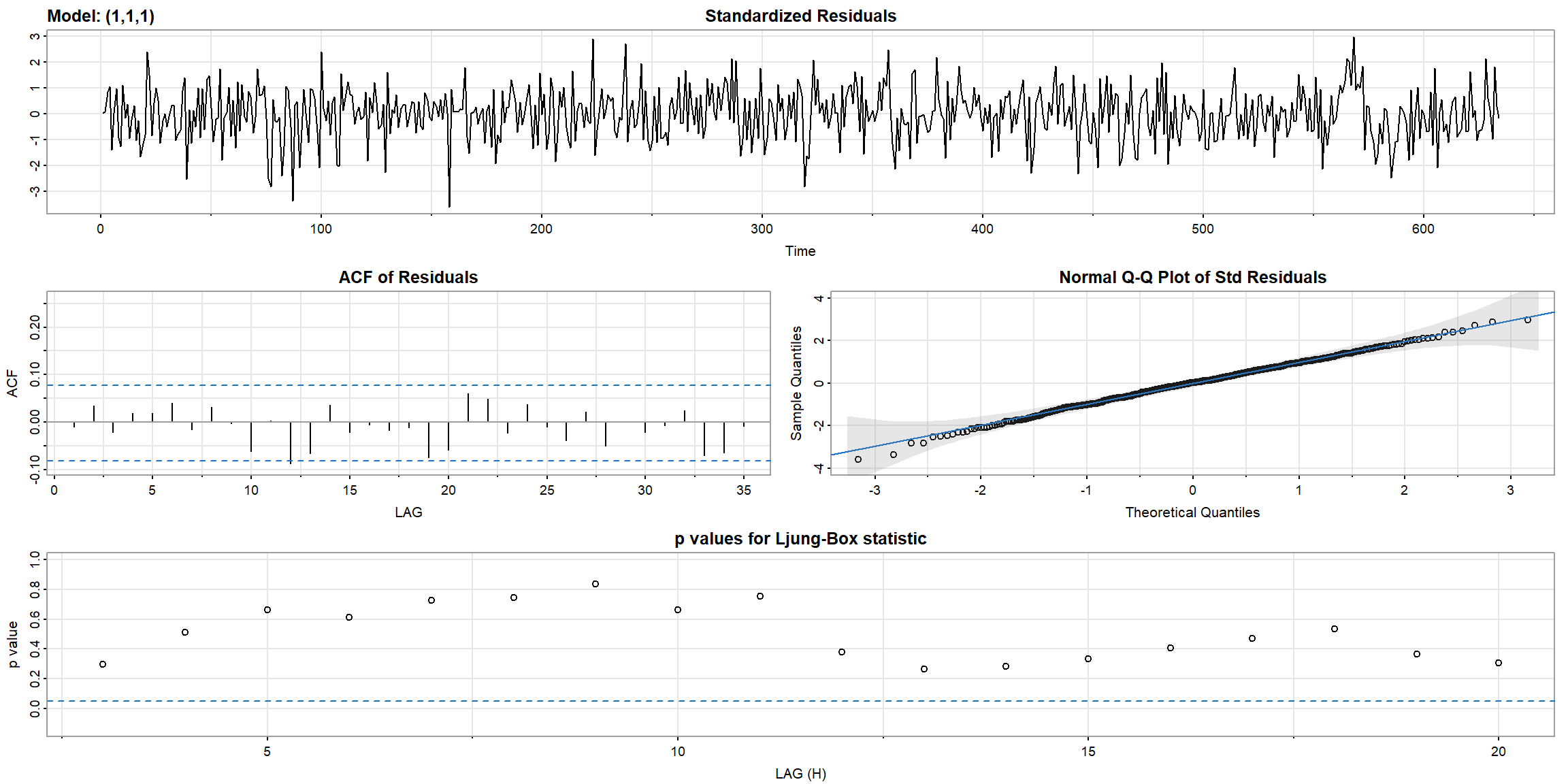
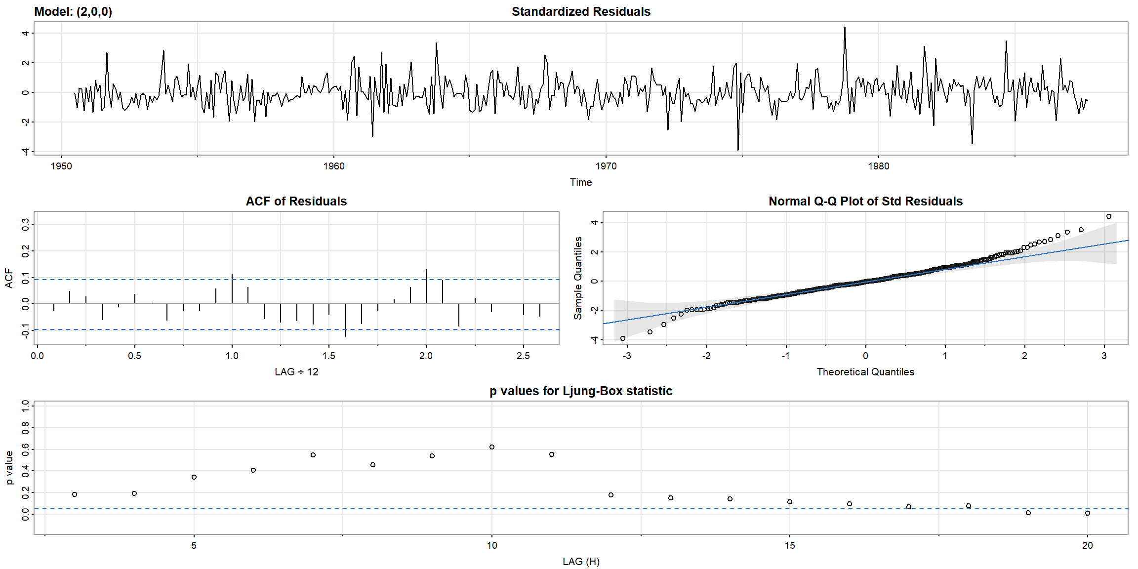
• all ACF inside the CI, and all p-value above 0.05, $\therefore$ ARIMA(1,1,1) is suitable for log(varve).

---

1.7 Regression with Autocorrelated Errors

Example 3.44 (p.144) Mortality, Temperature and Pollution

• 配適模型查看溫度(temperature)、顆粒物水平(particulate levels)與心血管死亡率(cardiovascular mortality)的關係

$$M_t=\beta_1+\beta_2t+\beta_3T_t+\beta_4T^2_t+\beta_5P_t+x_t$$

trend = time(cmort); temp = tempr - mean(tempr); temp2 = temp^2
fit <- lm(cmort~trend + temp + temp2 + part, na.action=NULL)
round(summary(fit)$coef, 3) |> knitr::kable()

	Estimate	Std. Error	t value	Pr(>|t|)
(Intercept)	2831.490	199.557	14.189	0
trend	-1.396	0.101	-13.820	0
temp	-0.472	0.032	-14.941	0
temp2	0.023	0.003	7.990	0
part	0.255	0.019	13.541	0

acf2(resid(fit), 52) # implies AR2

sarima(cmort, 2,0,0, xreg=cbind(trend,temp,temp2,part))

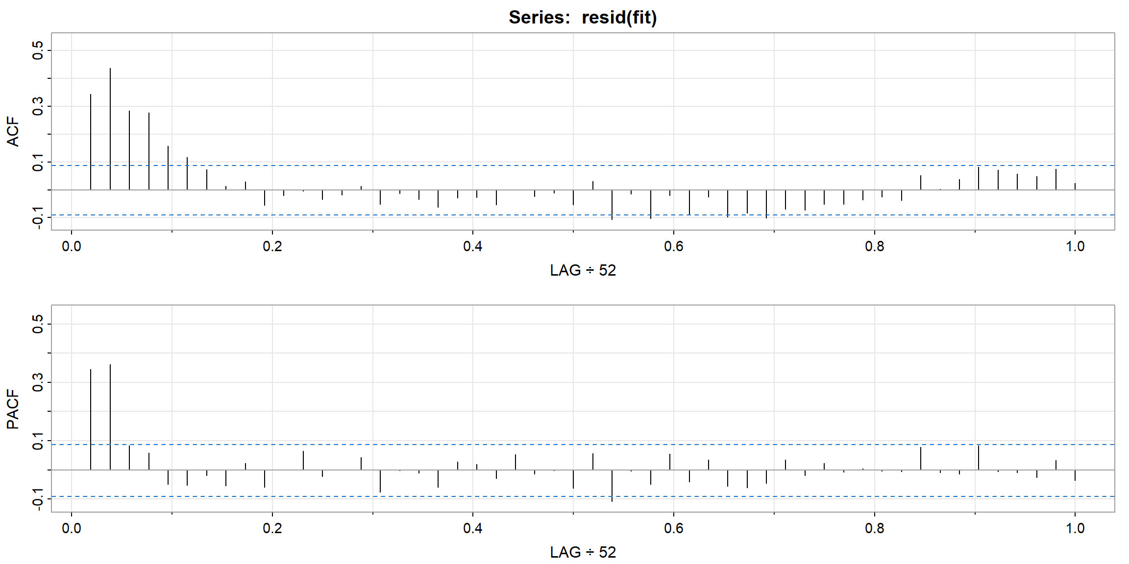
• ACF outside the CI, but the p-value are above 0.05, $\therefore$ AR(2) is not good enough for cmort.

---

Example 3.45 (p.145) Regression with Lagged Variables

$$R_t=\beta_0+\beta_1S_{t−6}+\beta_2D_{t−6}+\beta_3D_{t−6}S_{t−6}+wt$$

dummy = ifelse(soi<0, 0, 1)
fish = ts.intersect(rec, soiL6=lag(soi,-6), dL6=lag(dummy,-6), dframe=TRUE)
fit <- lm(rec ~ soiL6*dL6, data=fish, na.action=NULL)
round(summary(fit)$coef, 3) |> knitr::kable()

	Estimate	Std. Error	t value	Pr(>|t|)
(Intercept)	74.479	2.865	25.998	0.000
soiL6	-15.358	7.401	-2.075	0.039
dL6	-1.139	3.711	-0.307	0.759
soiL6:dL6	-51.244	9.523	-5.381	0.000

attach(fish)

## The following object is masked from package:astsa:
## 
##     rec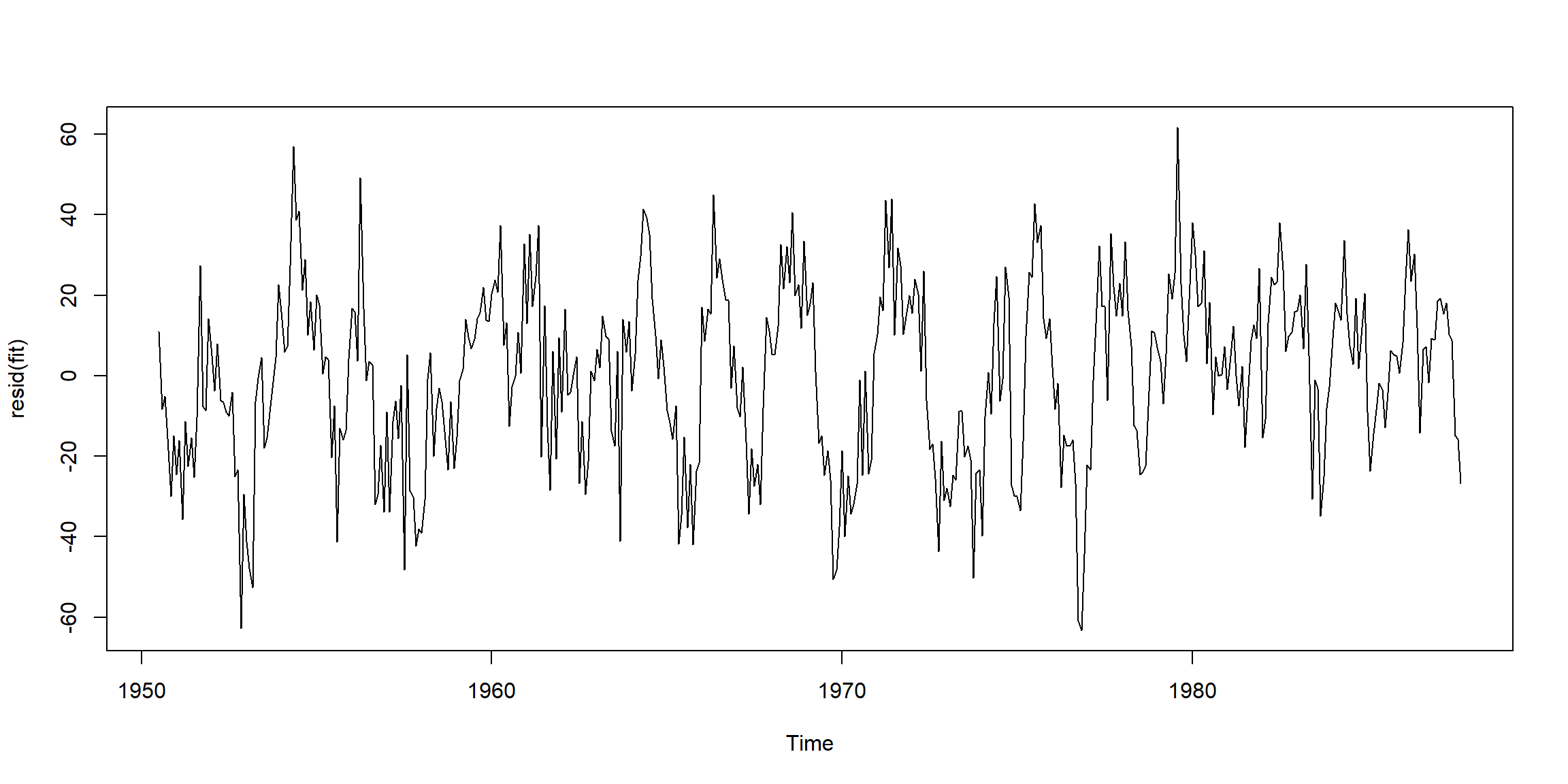

plot(resid(fit))

acf2(resid(fit)) # indicates AR(2)

intract = soiL6*dL6 # interaction term
sarima(rec,2,0,0, xreg = cbind(soiL6, dL6, intract))

• ACF outside the CI, and the p-value are below 0.05, $\therefore$ AR(2) is not suitable.

---

1.8 Multiplicative Seasonal ARIMA Models

• 先一階差分再看季節性 * 季節性資料優先處理季節性，再看需不需要差分

Example 3.46 (p.146) A Seasonal AR Series

$$(1 − 0.9\cdot B^{12})x_t = w_t$$

set.seed(666)
phi = c(rep(0,11),.9)
sAR = arima.sim(list(order=c(12,0,0), ar=phi), n=37)
sAR = ts(sAR, freq=12)
layout(matrix(c(1,1,2, 1,1,3), nc=2))
par(mar=c(3,3,2,1), mgp=c(1.6,.6,0))
plot(sAR, axes=FALSE, main='seasonal AR(1)', xlab="year", type='c')
Months = c("J","F","M","A","M","J","J","A","S","O","N","D")
points(sAR, pch=Months, cex=1.25, font=4, col=1:4)
axis(1, 1:4); abline(v=1:4, lty=2, col=gray(.7))
axis(2); box()
ACF = ARMAacf(ar=phi, ma=0, 100)
PACF = ARMAacf(ar=phi, ma=0, 100, pacf=TRUE)
plot(ACF,type="h", xlab="LAG", ylim=c(-.1,1)); abline(h=0)
plot(PACF, type="h", xlab="LAG", ylim=c(-.1,1)); abline(h=0)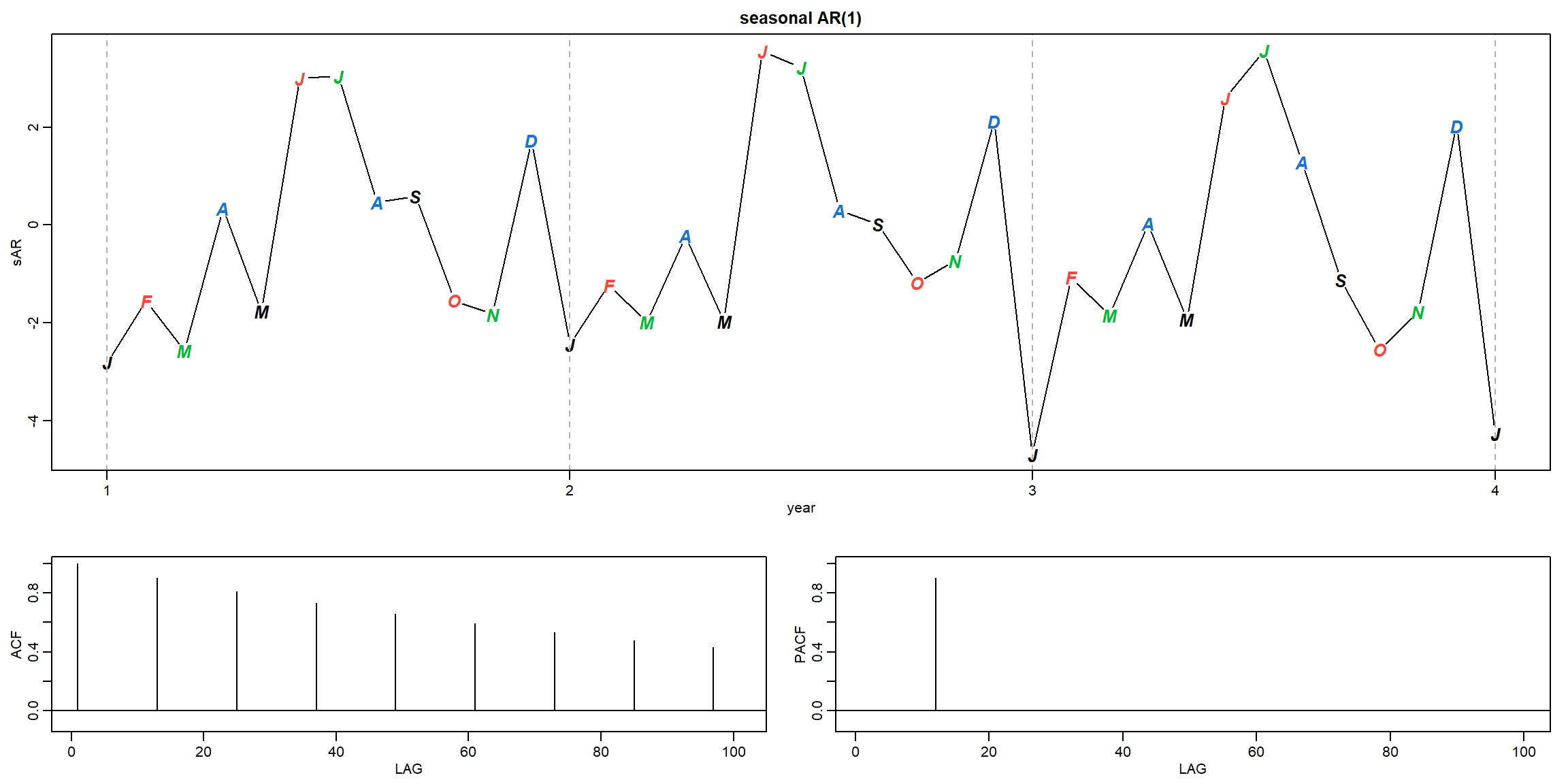

• Theoretical ACF tails off at lag 12, 24, 36, …
• Theoretical PACF cut-off at lag 12

acf2(sAR, max.lag = 35)

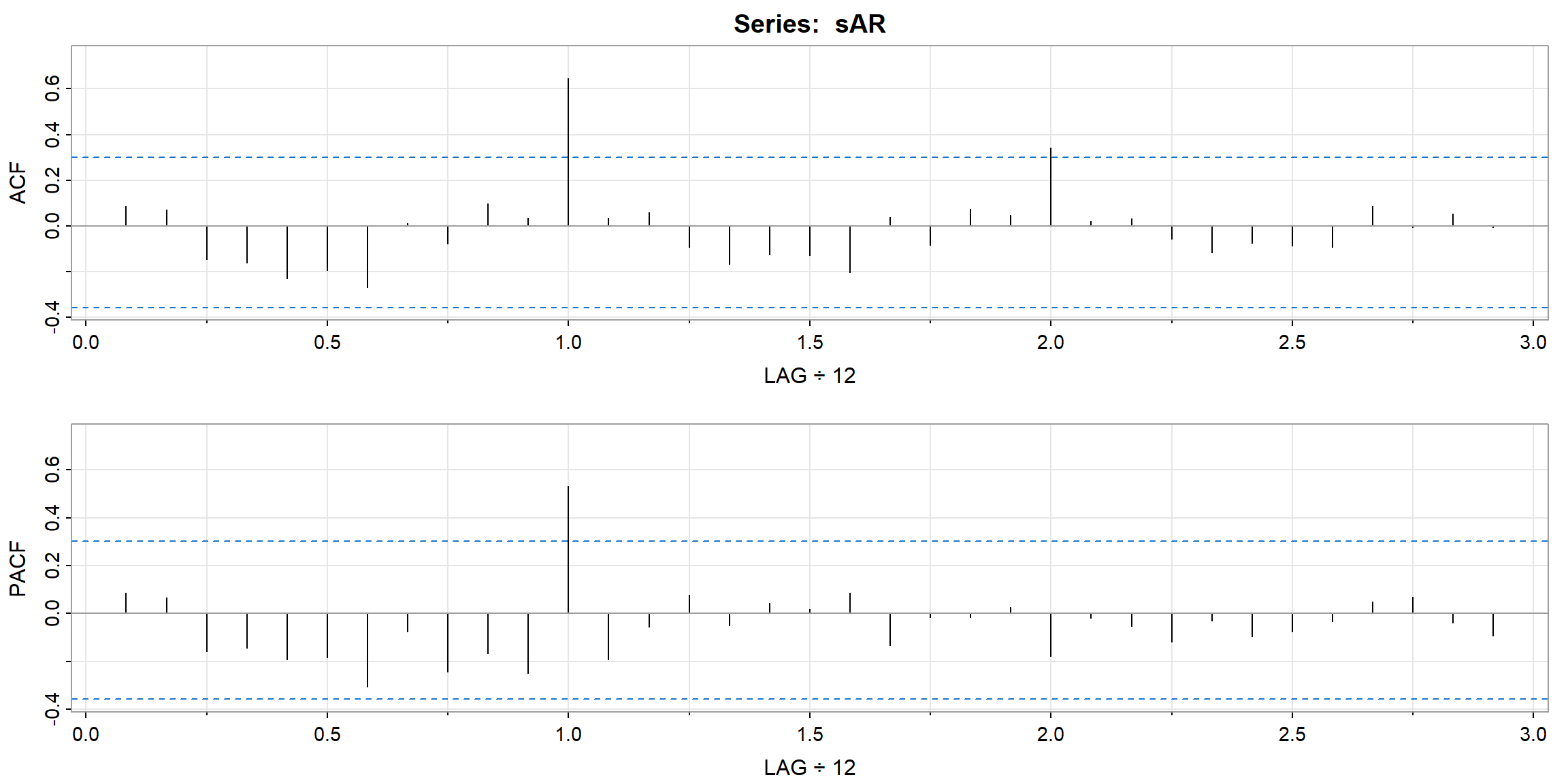
• Those patterns are also observed in the sample ACF and PACF.

---

Example 3.47 (p.145) seasonal ARMA

$$X_t-.8X_{t-12}=W_t-.5W_{t-1}$$

phi = c(rep(0,11),.8)
ACF = ARMAacf(ar=phi, ma=-.5, 50)[-1] # [-1] removes 0 lag
PACF = ARMAacf(ar=phi, ma=-.5, 50, pacf=TRUE)
par(mfrow=c(1,2))
plot(ACF, type="h", xlab="LAG", ylim=c(-.4,.8)); abline(h=0)
axis(1, at=0:50, label=F); axis(1, at=seq(0,50,by=10), lwd=2)
plot(PACF, type="h", xlab="LAG", ylim=c(-.4,.8)); abline(h=0)
axis(1, at=0:50, label=F); axis(1, at=seq(0,50,by=10), lwd=2)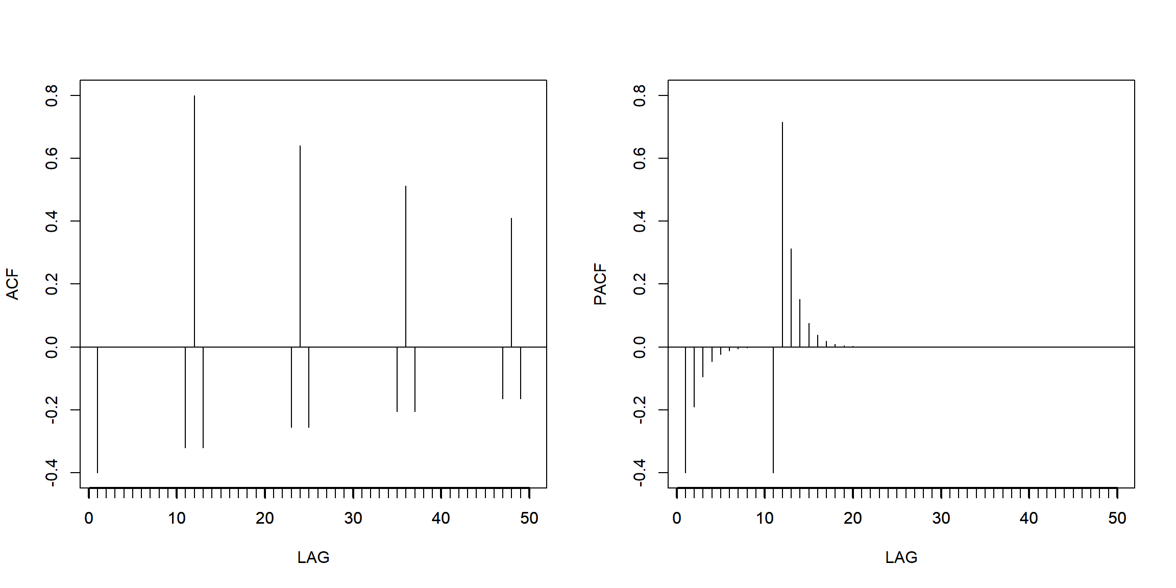

• PACF cut-off at lag 12, so $AR(1)_{12}$ is suitable.
• ACF cut-off at lag 1, so $MA(1)$ is suitable.

---

1.9 Periodogram

Example 4.1 (p.167) A Periodic Series

x1 = 2*cos(2*pi*1:100*6/100) + 3*sin(2*pi*1:100*6/100)
x2 = 4*cos(2*pi*1:100*10/100) + 5*sin(2*pi*1:100*10/100)
x3 = 6*cos(2*pi*1:100*40/100) + 7*sin(2*pi*1:100*40/100)
x = x1 + x2 + x3

par(mfrow=c(2,2), mar=c(4,4,2,1))
plot.ts(x1, ylim=c(-10,10), main=expression(omega==6/100~~~A^2==13))
plot.ts(x2, ylim=c(-10,10), main=expression(omega==10/100~~~A^2==41))
plot.ts(x3, ylim=c(-10,10), main=expression(omega==40/100~~~A^2==85))
plot.ts(x, ylim=c(-16,16), main="sum")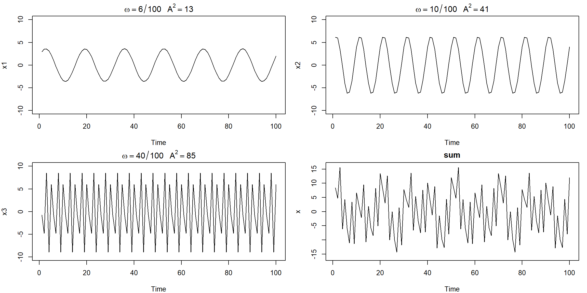

when there is many periodic, it is hard to see

• A: height of the peak
  • for $x_1$, $A^2=2^2+3^2=13$, the maximum and minimum values that $x_1$ will attain are $\pm\sqrt{13}=\pm3.61$
• $\omega=\frac jn$: j = repeated times

---

Example 4.2 (p.169) Estimation and the Periodogram

P = Mod(2*fft(x)/100)^2; Fr = 0:99/100
plot(Fr, P, type="o", xlab="frequency", ylab="scaled periodogram")
abline(v=0.5, col="red", lty=2)
points(x=Fr[7], y=P[7], col="red", pch=1, cex=3);text(x=Fr[7], y=P[7], labels = "6/100", pos=3, col="red")
points(x=Fr[11], y=P[11], col="red", pch=1, cex=3);text(x=Fr[11], y=P[11], labels = "10/100", pos=3, col="red")
points(x=Fr[41], y=P[41], col="red", pch=1, cex=3);text(x=Fr[41], y=P[41], labels = "40/100", pos=1, col="red")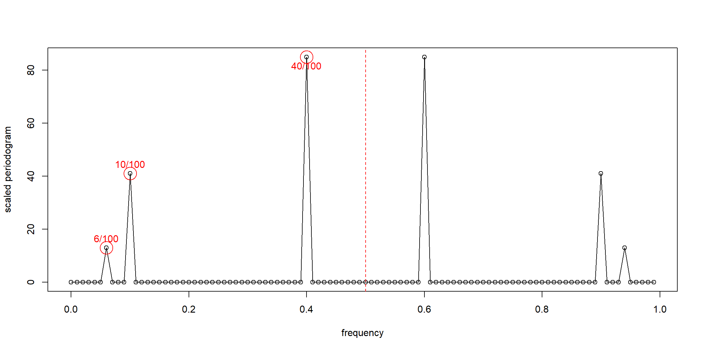

• the plot is symmetric: $I(\omega_j)=I(\omega_{n-j})$
• period: $T=\frac nj$
  • $T_1=\frac {100}6$, $T_2=\frac{100}{10}$, $T_3=\frac{100}{40}$
• $\omega_j=\frac jn$
  • $\omega_1=\frac 6{100}$, $\omega_2=\frac {10}{100}$, $\omega_3=\frac {40}{100}$

---

Example 4.7 (p.176) spectral density

par(mfrow=c(3,1), mar=c(4,4,1,1))
arma.spec(main="White Noise")
arma.spec(ma=.5, main="Moving Average")
arma.spec(ar=c(1,-.9), main="Autoregression")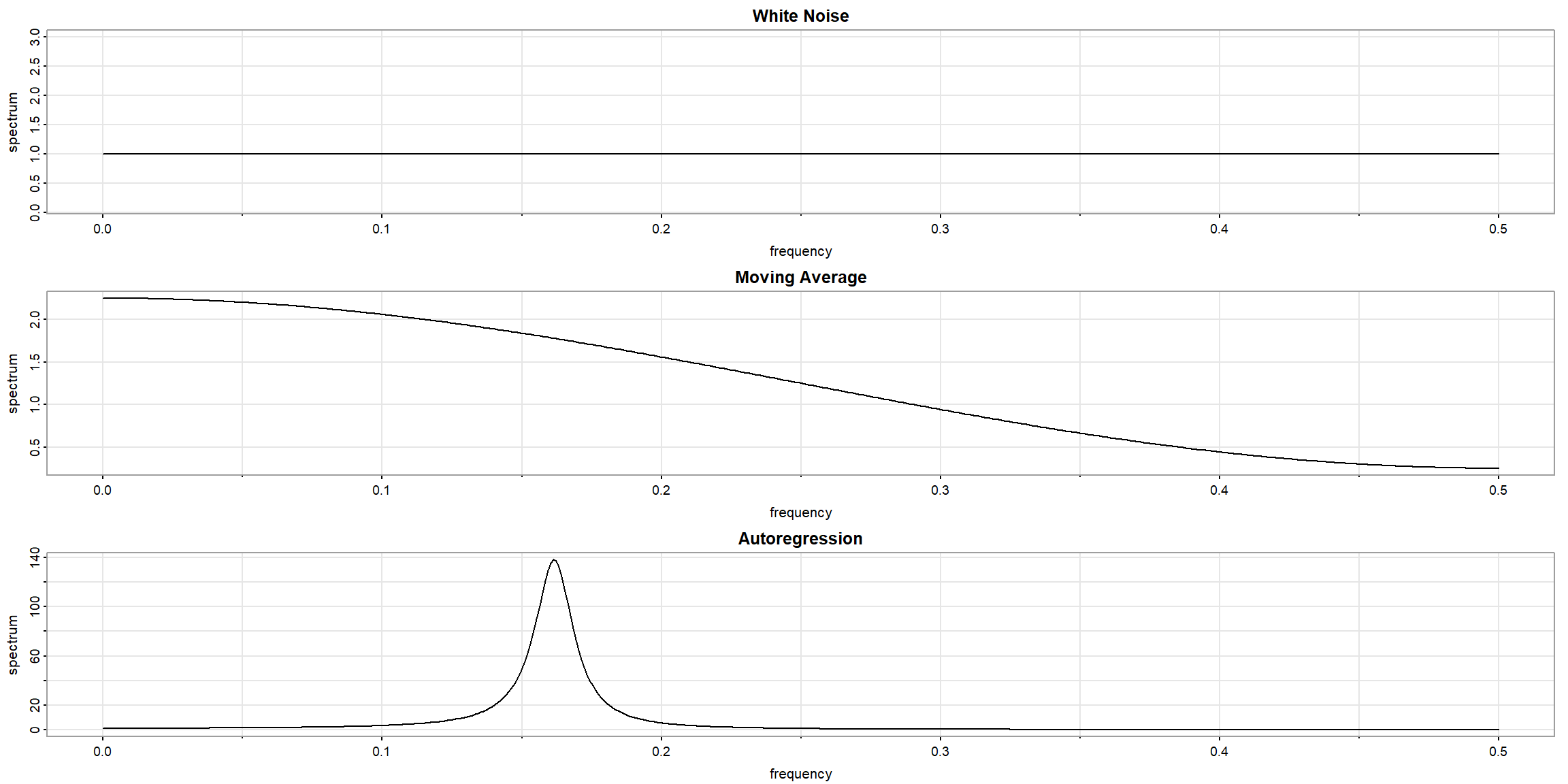

• Top: White Noise
• Middle: MA(1), $\theta_1=0.5$
• Bottom: AR(2), $\phi_1=1, \phi_2=-0.9$

---

Example 4.10 (p.182) Spectral ANOVA

periodogram is symmetric

$$\omega_1=\frac15,\omega_2=\frac25$$

$$SS=2\cdot I(\omega_j)$$

x = c(1, 2, 3, 2, 1)
c1 = cos(2*pi*1:5*1/5); s1 = sin(2*pi*1:5*1/5)
c2 = cos(2*pi*1:5*2/5); s2 = sin(2*pi*1:5*2/5)
omega1 = cbind(c1, s1); omega2 = cbind(c2, s2)
anova(lm(x~omega1+omega2)) # ANOVA Table

## Analysis of Variance Table
## 
## Response: x
##           Df  Sum Sq Mean Sq F value Pr(>F)
## omega1     2 2.74164 1.37082     NaN    NaN
## omega2     2 0.05836 0.02918     NaN    NaN
## Residuals  0 0.00000     NaN

• $2.74=2\cdot I(\frac15)=2\cdot1.37$

$\downarrow$ $I(0)$ $I(\frac15)$ $I(\frac25)$ $I(\frac35)$ $I(\frac45)$

Mod(fft(x))^2/5 # the periodogram (as a check)

## [1] 16.20000000  1.37082039  0.02917961  0.02917961  1.37082039

---

Example 4.13 (p.187) CI

• n=480, $\because$ periodogram is symmatric, only need to print half of them
• 1 unit = 40

par(mfrow=c(2,1), mar=c(4,4,1,1))
soi.per = mvspec(soi, log="no")
abline(v=1/4, lty=2)
rec.per = mvspec(rec, log="no")
abline(v=1/4, lty=2)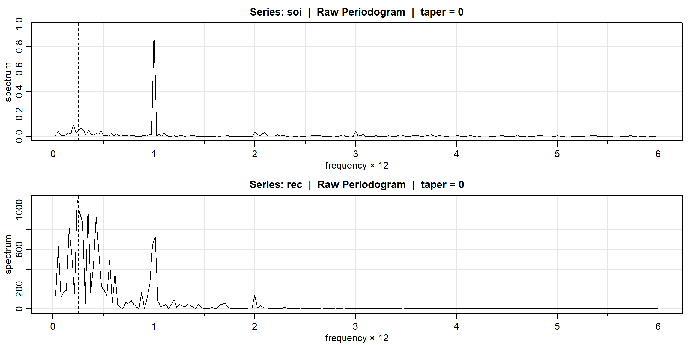

• the peak appear at j=10, 40

---

$$\frac{2I(\omega_j)}{f(\omega_j)}\sim\chi^2(2)$$

$$\text{95% CI for }f(\omega_j)=[\frac{2I(\omega_j)}{\chi^2_.975}, \frac{2I(\omega_j)}{\chi^2_.025}]$$

• $\downarrow I(\omega_j)$

soi.per$spec[40] # 0.97223; soi pgram at freq 1/12 = 40/480
soi.per$spec[10] # 0.05372; soi pgram at freq 1/48 = 10/480

## [1] 0.9722312
## [1] 0.05372962

• $\downarrow CI$: huge interval is a useless interval

U = qchisq(.025,2) # 0.05063
L = qchisq(.975,2) # 7.37775

2*soi.per$spec[10]/L # 0.01456
2*soi.per$spec[10]/U # 2.12220

2*soi.per$spec[40]/L # 0.26355
2*soi.per$spec[40]/U # 38.40108

## [1] 0.0145653
## [1] 2.122207
## [1] 0.2635573
## [1] 38.40108