Chapter 8 GWAS
8.1 GWAS analysis
In this exercise, we are conducting a GWAS for four different models: 1) Naive (T-test), 2) GLM accounting for population structure (Q), 3) MLM accounting for population structure (Q) and Kinship (K), 4) FarmCPU accounting for population structure (Q) and Kinship (K). Each model is testing the same hypothesis: Ho: No association between SNP and trait. Ha: There is an association between SNP and trait.
The Naive model is fit using base R functions and GLM, MLM and FarmCPU models are run using the rMVP R package (Yin et al. 2021).
Additional packages used in this section are data.table (Dowle and Srinivasan 2021), and tidyverse (Wickham 2021).
Load necessary packages
library(rMVP)
library(data.table)
library(tidyverse)
Set working directory to where rMVP files are in workshop materials
setwd("~/PGRP_mapping_workshop/data/genotypic_and_phenotypic_data/")Read in phenotypes
phenos = fread("WIDIV_942.phe", data.table = FALSE)Read in SNPs
myGD = attach.big.matrix("WIDIV_942.geno.desc")Read in SNPs map
map = fread("WIDIV_942.geno.map", data.table = FALSE)Read in Kinship matrix (A matrix)
myKin = attach.big.matrix("WIDIV_942.kin.desc")Read in principle components (Q)
snp_pcs = attach.big.matrix("WIDIV_942.pc.desc")
snp_pcs = snp_pcs[,]
Run a naive model without any correction for kinship or population structure
### Make a dataframe with phenotypes and genotypes together
GD_naive = cbind(phenos,t(myGD[,]))

### Fit a simple linear regression model for low heritability simulated trait regressed on SNPs and save those results for later
low_h2_naive = sapply(4:ncol(GD_naive), function(x) anova(lm(GD_naive$Color_low_h2 ~ GD_naive[,x]))$'Pr(>F)'[1])
low_h2_naive = cbind(map,low_h2_naive)
colnames(low_h2_naive)[6] = "Color_low_h2.Naive"

### Fit a simple linear regression model for high heritability simulated trait regressed on SNPs
high_h2_naive = sapply(4:ncol(GD_naive), function(x) anova(lm(GD_naive$Color_high_h2 ~ GD_naive[,x]))$'Pr(>F)'[1])
high_h2_naive = cbind(map,high_h2_naive)
colnames(high_h2_naive)[6] = "Color_high_h2.Naive"

### Save those results for visualizing later with IGV
setwd("~/PGRP_mapping_workshop/gwas_results/for_IGV_visualization/")
low_h2_naive_IGV = low_h2_naive[,c(2,3,1,6)]
colnames(low_h2_naive_IGV) = c("CHR","BP","SNP","P")
high_h2_naive_IGV = high_h2_naive[,c(2,3,1,6)]
colnames(high_h2_naive_IGV) = c("CHR","BP","SNP","P")
fwrite(low_h2_naive_IGV, file = "Color_low_h2_naive.gwas",col.names = TRUE, sep = "\t", quote = FALSE, na = "NA")
fwrite(high_h2_naive_IGV, file = "Color_high_h2_naive.gwas",col.names = TRUE, sep = "\t", quote = FALSE, na = "NA")

## Save results for simple static plot visualization later
setwd("~/PGRP_mapping_workshop/gwas_results/")
fwrite(low_h2_naive, file = "Color_low_h2_naive.txt",col.names = TRUE, sep = "\t", quote = FALSE, na = "NA")
fwrite(high_h2_naive, file = "Color_high_h2_naive.txt",col.names = TRUE, sep = "\t", quote = FALSE, na = "NA")
Run GLM with (Q), MLM with (Q) and (K), and FarmCPU with (Q) and (K) and save results for IGV visualization Note to visualize gwas results in IGV, you need a .gwas file which has four columns, CHR, SNP, BP, and P. The loop below writes the .gwas file for each model fit to the high heritability trait and the low heritability trait.
setwd("~/PGRP_mapping_workshop/gwas_results/for_IGV_visualization/")
for(i in colnames(phenos)[2:ncol(phenos)]){
  gwas_kinship = MVP(
    phe=phenos[, c("Taxa", i)], # Phenotype dataframe
    geno=myGD, # Genotypic data as a big.matrix
    map=map, # Map dataframe
    K=myKin, # Kinship used in MLM
    maxLoop=10, # Max number of iterations for FarmCPU
    CV.GLM=snp_pcs[,1:3], # Covariates (Q) in GLM
    CV.MLM=snp_pcs[,1:3], # Covariates (Q) in MLM
    CV.FarmCPU=snp_pcs[,1:3], # Covariates (Q) in FarmCPU
    method.bin="FaST-LMM", # Method for optimizing bins used by FarmCPU
    method=c("GLM", "MLM", "FarmCPU"), # GWAS models being fit
    file.output = FALSE # If set to TRUE, will generate many plots and files for each trait
  )
  ### These lines are simply for reformatting and remove columns which you would normally want to keep for real data such as effect sizes and standard error associated with each test.
  GLM = cbind(gwas_kinship$map,gwas_kinship$glm.results)
  GLM = GLM[,c(2,3,1,8)]
  colnames(GLM) = c("CHR","BP","SNP","P")
  fwrite(GLM, file = paste0(i,"_GLM_Q.gwas"),col.names = TRUE, sep = "\t", quote = FALSE, na = "NA")
  MLM = cbind(gwas_kinship$map,gwas_kinship$mlm.results)
  MLM = MLM[,c(2,3,1,8)]
  colnames(MLM) = c("CHR","BP","SNP","P")
  fwrite(MLM, file = paste0(i,"_MLM_QandK.gwas"),col.names = TRUE, sep = "\t", quote = FALSE, na = "NA")
  CPU = cbind(gwas_kinship$map,gwas_kinship$farmcpu.results)
  CPU = CPU[,c(2,3,1,8)]
  colnames(CPU) = c("CHR","BP","SNP","P")
  fwrite(CPU, file = paste0(i,"_FarmCPU_QandK.gwas"),col.names = TRUE, sep = "\t", quote = FALSE, na = "NA")
  gc()
}
Run the same models, but saving output to a text file for static visualization later
setwd("~/PGRP_mapping_workshop/gwas_results/")
for(i in colnames(phenos)[2:ncol(phenos)]){
  gwas_kinship = MVP(
    phe=phenos[, c("Taxa", i)],
    geno=myGD,
    map=map,
    K=myKin,
    CV.GLM=snp_pcs[,1:3],
    CV.MLM=snp_pcs[,1:3],
    CV.FarmCPU=snp_pcs[,1:3],
    maxLoop=10,
    method.bin="FaST-LMM",
    method=c("GLM", "MLM", "FarmCPU"),
    file.output = FALSE
  )
  GLM = cbind(gwas_kinship$map,gwas_kinship$glm.results)
  GLM = GLM[,-c(6:7)]
  colnames(GLM)[6] = paste0(colnames(GLM)[6],".Q")
  fwrite(GLM, file = paste0(i,"_GLM_Q.txt"),col.names = TRUE, sep = "\t", quote = FALSE, na = "NA")
  MLM = cbind(gwas_kinship$map,gwas_kinship$mlm.results)
  MLM = MLM[,-c(6:7)]
  colnames(MLM)[6] = paste0(colnames(MLM)[6],".QandK")
  fwrite(MLM, file = paste0(i,"_MLM_QandK.txt"),col.names = TRUE, sep = "\t", quote = FALSE, na = "NA")
  CPU = cbind(gwas_kinship$map,gwas_kinship$farmcpu.results)
  CPU = CPU[,-c(6:7)]
  colnames(CPU)[6] = paste0(colnames(CPU)[6],".QandK")
  fwrite(CPU, file = paste0(i,"_FarmCPU_QandK.txt"),col.names = TRUE, sep = "\t", quote = FALSE, na = "NA")
  gc()
}
8.2 Static plot visualization
Now that the analysis has been run, lets visualize the results in a static manhattan plot. For this we will use the CMplot R package (R-CMplot?). These plots are saved in the directory set below.
Load necessary packages
library(CMplot)Read in the results which were saved to individual text files
setwd("~/PGRP_mapping_workshop/gwas_results/")
gwas_results_files = list.files() # Lists the files in the directory
gwas_results_files = gwas_results_files[!gwas_results_files%in%c("for_IGV_visualization")] # Remove the "for_IGV_visualisation"

gwas_results = list() # Make a list for the dataframes to be read into

## This loop reads in the results into a list. Each element of the list is a dataframe with the results for the model fit
for (i in gwas_results_files){
  gwas_results[[i]] = fread(i)
}
Combine the results from a list into a single dataframe
all.results.pvals = gwas_results %>%
  reduce(left_join, by = c("SNP","CHROM","POS","REF","ALT"))
all.results.pvals = data.frame(all.results.pvals)
Set the working directory to where the figures will be saved
setwd("~/PGRP_mapping_workshop/figures/gwas/")Set the bonferroni correction at alpha = 0.05
bonf = 0.05/nrow(all.results.pvals)Plot for high heritability trait models
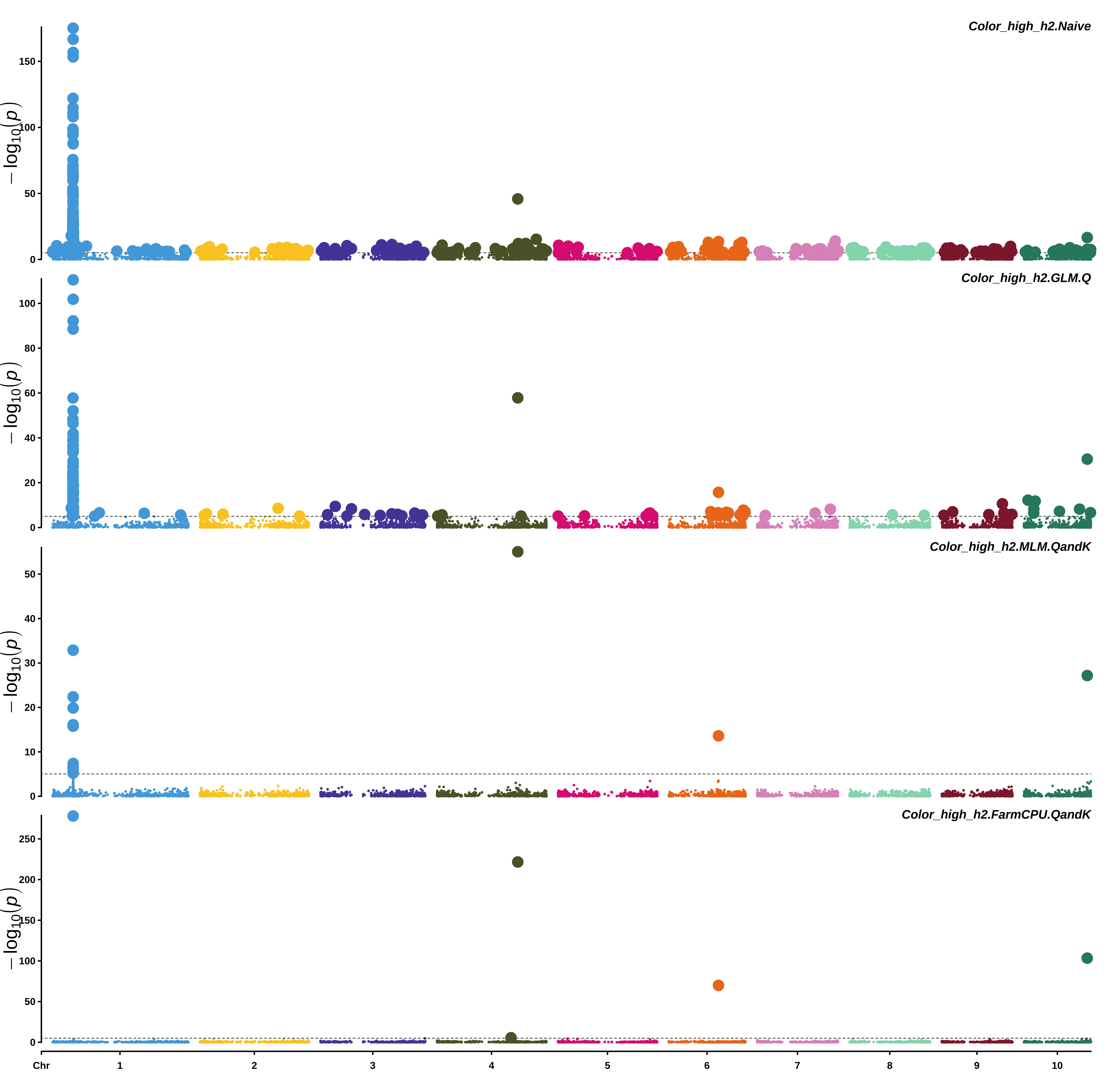
high_models =  all.results.pvals[,c("SNP","CHROM","POS",
                                    "Color_high_h2.Naive","Color_high_h2.GLM.Q",
                                    "Color_high_h2.MLM.QandK","Color_high_h2.FarmCPU.QandK")]

plot_high_models = CMplot(high_models,
                    band = 1.2,
                    cex.axis = 2,
                    plot.type=c("m","q"),
                    multracks = TRUE,
                    cex = 0.4,
                    threshold=bonf,
                    threshold.col="black",
                    threshold.lwd=1.25,
                    threshold.lty=2,
                    signal.cex=1.25,
                    LOG10=TRUE,
                    box=FALSE,
                    width=25,
                    ## Other options
                    chr.den.col=c("darkgreen", "yellow", "red"),
                    cex.lab= 2,
                    file.output=TRUE,
                    verbose=TRUE,
                    memo = "HIGH_models")
From top to bottom, manhattan plots are for a Naive model (T-test), GLM model accounting for (Q), MLM model accounting for (Q) and (K), FarmCPU model accounting for (Q) and (K).
Plot for low heritability trait models
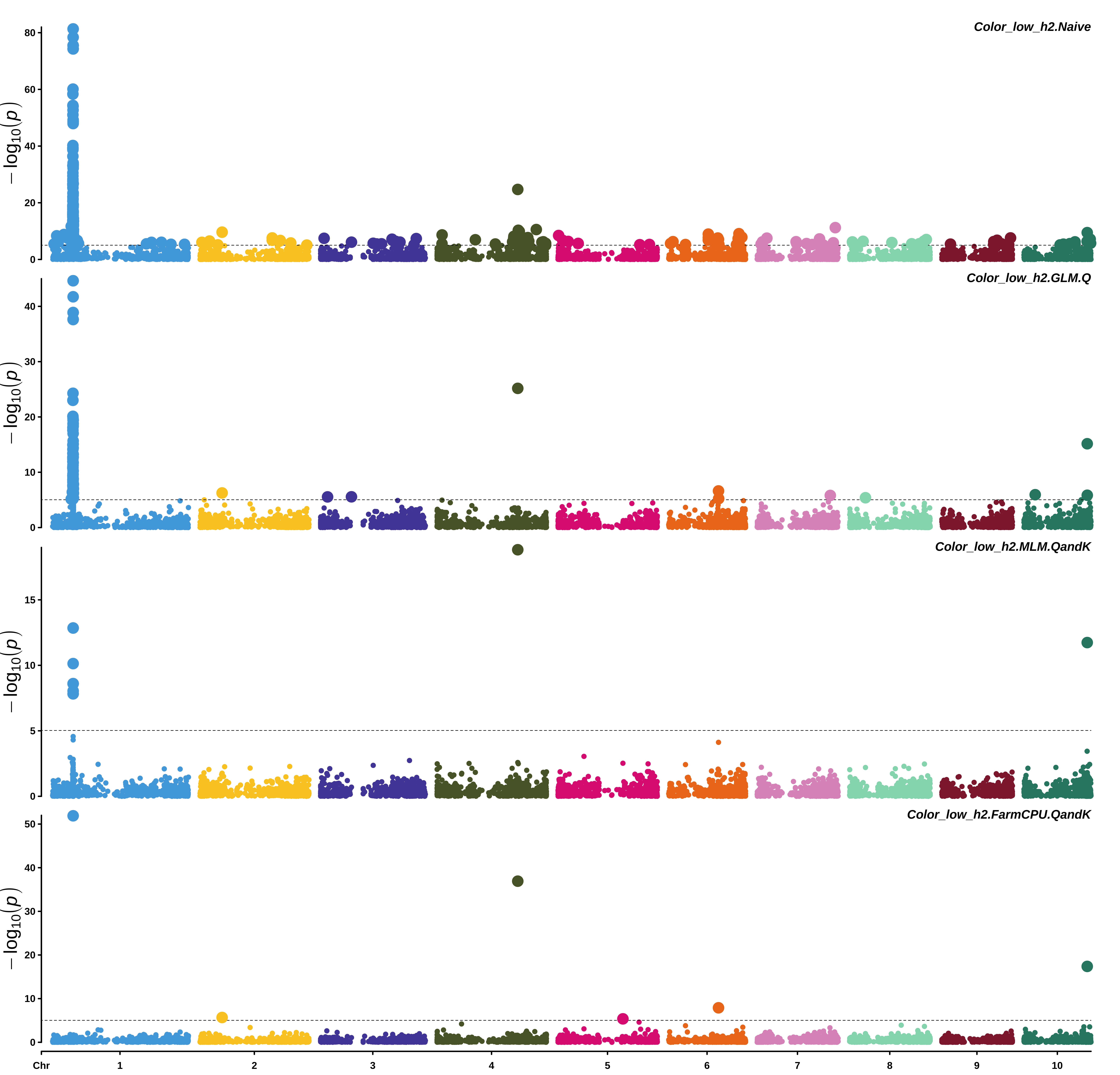
low_models =  all.results.pvals[,c("SNP","CHROM","POS",
                                   "Color_low_h2.Naive","Color_low_h2.GLM.Q",
                                   "Color_low_h2.MLM.QandK","Color_low_h2.FarmCPU.QandK")]

plot_low_models = CMplot(low_models,
                          band = 1.2,
                          cex.axis = 2,
                          plot.type=c("m","q"),
                          multracks = TRUE,
                          cex = 0.9,
                          threshold=bonf,
                          threshold.col="black",
                          threshold.lwd=1.25,
                          threshold.lty=2,
                          signal.cex=1.25,
                          LOG10=TRUE,
                          box=FALSE,
                          width=25,
                          ## Other options
                          chr.den.col=c("darkgreen", "yellow", "red"),
                          cex.lab= 2,
                          file.output=TRUE,
                          verbose=TRUE,
                          memo = "LOW_models")
From top to bottom, manhattan plots are for a Naive model (T-test), GLM model accounting for (Q), MLM model accounting for (Q) and (K), FarmCPU model accounting for (Q) and (K).
As a reminder, these are the QTLs we simulated.