Chapter 7 Data Merging
Hello! In this tutorial, we will go over some data wrangling strategies when dealing with two or more datasets. Let’s begin by loading in the appropriate packages (mainly, tidyverse).
options(scipen=999) #use this to remove scientific notation

library(plyr)
library(tidyverse)
Alrighty! Let’s now download our data. For this analysis, we will be looking at two datasets: (1) a list of NYT articles about COVID (not the actual stories, but headlines, URLs, and meta-data) and (2) U.S. COVID-19 data (cases, deaths).
data_covid <- read_csv("data/covid_cases.csv") #don't forget to make sure these files are in your working directory!
data_nyt <- read_csv("data/covid_nyt_stories.csv")
Let’s first use str() and head() to see what’s in the data.
str(data_covid)## spec_tbl_df [385 x 8] (S3: spec_tbl_df/tbl_df/tbl/data.frame)
## $ iso_code : chr [1:385] "USA" "USA" "USA" "USA" ...
## $ date : chr [1:385] "1/22/2020" "1/23/2020" "1/24/2020" "1/25/2020" ...
## $ total_cases : num [1:385] 1 1 2 2 5 5 5 6 6 8 ...
## $ new_cases : num [1:385] NA 0 1 0 3 0 0 1 0 2 ...
## $ total_deaths : num [1:385] NA NA NA NA NA NA NA NA NA NA ...
## $ new_deaths : num [1:385] NA NA NA NA NA NA NA NA NA NA ...
## $ total_cases_per_million: num [1:385] 0.003 0.003 0.006 0.006 0.015 0.015 0.015 0.018 0.018 0.024 ...
## $ new_cases_per_million : num [1:385] NA 0 0.003 0 0.009 0 0 0.003 0 0.006 ...
## - attr(*, "spec")=
## .. cols(
## .. iso_code = col_character(),
## .. date = col_character(),
## .. total_cases = col_double(),
## .. new_cases = col_double(),
## .. total_deaths = col_double(),
## .. new_deaths = col_double(),
## .. total_cases_per_million = col_double(),
## .. new_cases_per_million = col_double()
## .. )
## - attr(*, "problems")=<externalptr>str(data_nyt)## spec_tbl_df [28,350 x 10] (S3: spec_tbl_df/tbl_df/tbl/data.frame)
## $ stories_id : num [1:28350] 1490114687 1491992217 1496159739 1497814035 1498707611 ...
## $ publish_date : POSIXct[1:28350], format: "2020-01-08 21:48:29" "2020-01-10 20:41:55" ...
## $ title : chr [1:28350] "China Identifies New Virus Causing Pneumonia-Like Illness" "China Reports First Death From New Virus" "Japan Confirms First Case of New Chinese Coronavirus" "Three U.S. Airports to Screen Passengers for Chinese Coronavirus" ...
## $ url : chr [1:28350] "https://www.nytimes.com/2020/01/08/health/china-pneumonia-outbreak-virus.html" "https://www.nytimes.com/2020/01/10/world/asia/china-virus-wuhan-death.html" "https://www.nytimes.com/2020/01/15/world/asia/coronavirus-japan-china.html" "https://www.nytimes.com/2020/01/17/health/china-coronavirus-airport-screening.html" ...
## $ language : chr [1:28350] "en" "en" "en" "en" ...
## $ ap_syndicated: logi [1:28350] FALSE FALSE FALSE FALSE FALSE FALSE ...
## $ themes : chr [1:28350] NA NA NA NA ...
## $ media_id : num [1:28350] 1 1 1 1 1 1 1 1 1 1 ...
## $ media_name : chr [1:28350] "New York Times" "New York Times" "New York Times" "New York Times" ...
## $ media_url : chr [1:28350] "http://nytimes.com" "http://nytimes.com" "http://nytimes.com" "http://nytimes.com" ...
## - attr(*, "spec")=
## .. cols(
## .. stories_id = col_double(),
## .. publish_date = col_datetime(format = ""),
## .. title = col_character(),
## .. url = col_character(),
## .. language = col_character(),
## .. ap_syndicated = col_logical(),
## .. themes = col_character(),
## .. media_id = col_double(),
## .. media_name = col_character(),
## .. media_url = col_character()
## .. )
## - attr(*, "problems")=<externalptr>head(data_covid$date)## [1] "1/22/2020" "1/23/2020" "1/24/2020" "1/25/2020" "1/26/2020" "1/27/2020"head(data_nyt$publish_date)## [1] "2020-01-08 21:48:29 UTC" "2020-01-10 20:41:55 UTC"
## [3] "2020-01-15 22:30:04 UTC" "2020-01-17 14:08:42 UTC"
## [5] "2020-01-18 22:08:02 UTC" "2020-01-20 05:59:15 UTC"str(data_nyt$publish_date)## POSIXct[1:28350], format: "2020-01-08 21:48:29" "2020-01-10 20:41:55" "2020-01-15 22:30:04" ...Of the 8 variables in the COVID dataset and the 10 variables in the NYT dataset, it’s worth noting that one variable they kind of share in common is time. So, it might be interesting to construct a plot of the number of cases and number of articles about COVID daily. To do this, we’ll have to merge these two datasets.
But these datasets are in slightly different structures. data_covid is daily data, whereas the data_nyt dataset is at the article-level with both date and timestamp information included in the publish_date variable. So, before we merge, we need to learn more about how to wrangle both datasets.
7.1 More Data Types
7.1.1 Datetime
So “datetimes” are variable-types that include date and time information (in R, you can construct both date and datetime variables). In R, they follow the following structure: YYYY-MM-DD HH:MM:SS. Base R calls this type of data a POSIXct.
head(data_nyt$publish_date)## [1] "2020-01-08 21:48:29 UTC" "2020-01-10 20:41:55 UTC"
## [3] "2020-01-15 22:30:04 UTC" "2020-01-17 14:08:42 UTC"
## [5] "2020-01-18 22:08:02 UTC" "2020-01-20 05:59:15 UTC"str(data_nyt$publish_date)## POSIXct[1:28350], format: "2020-01-08 21:48:29" "2020-01-10 20:41:55" "2020-01-15 22:30:04" ...One nice thing about datetime variables is that you can subtract datetime variables from one another (but you can’t do other operations, which makes sense because you can’t divide last week by tomorrow).
data_nyt$publish_date[1]## [1] "2020-01-08 21:48:29 UTC"data_nyt$publish_date[2]## [1] "2020-01-10 20:41:55 UTC"data_nyt$publish_date[2] - data_nyt$publish_date[1]## Time difference of 1.953773 days#data_nyt$publish_date[2] * data_nyt$publish_date[1] this line will not work7.1.2 Dates
In the data_covid dataset, we have a Date variable, but it’s not actually a date (you’ll see this if you use str())
str(data_covid$date)## chr [1:385] "1/22/2020" "1/23/2020" "1/24/2020" "1/25/2020" "1/26/2020" ...So, we’ll need to coerce this variable into a date variable. We can do so using the as.Date() function.
If your character/string is already structured like this: "2020-01-10", then as.Date() will interpret this easily. In most cases, though, we often have to tell R what the format of the Date (or datetime) structure is. We can do this using the format() argument in the as.Date() function (here, we will use "%m/%d/%Y", representing:
data_covid$date <- as.Date(data_covid$date, format = "%m/%d/%Y")
str(data_covid$date)
## Date[1:385], format: "2020-01-22" "2020-01-23" "2020-01-24" "2020-01-25" "2020-01-26" ...head(data_covid$date)## [1] "2020-01-22" "2020-01-23" "2020-01-24" "2020-01-25" "2020-01-26"
## [6] "2020-01-27"data_nyt$publish_date <- as.Date(data_nyt$publish_date)
str(data_nyt$publish_date)## Date[1:28350], format: "2020-01-08" "2020-01-10" "2020-01-15" "2020-01-17" "2020-01-18" ...When plotting datetimes and dates, ggplot2 will also organize the axis nicely.
ggplot(data_covid, aes(x = date, y = new_deaths)) +
  geom_line() +
  labs(title = "Number of new COVID-19 Deaths, Daily", x = "Date", y = "Number of deaths") +
  theme_minimal()
## Warning: Removed 38 row(s) containing missing values (geom_path).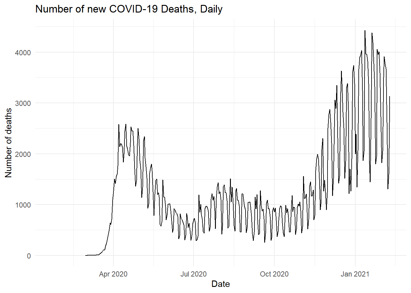 Now, let’s take a very brief detour to talk about strings.
7.1.3 Strings
The data_nyt dataset is a good opportunity to give you a primer on dealing with strings/characters. As I’ve mentioned, strings and characters are types of data that scholars use to work with text data. Computers are not great at understanding language (in fact, without human involvement, they don’t understand language), but they are great for repetitive pattern recognition. For that reason, it can be very easy to identify parts of a string (like a keyword or consisent phrase), replace it, or search y it.
For the next few lines, let’s focus on the title variable in the data_nyt dataset.
7.1.3.1 With base R
head(data_nyt$title, n = 10)## [1] "China Identifies New Virus Causing Pneumonia-Like Illness"
## [2] "China Reports First Death From New Virus"
## [3] "Japan Confirms First Case of New Chinese Coronavirus"
## [4] "Three U.S. Airports to Screen Passengers for Chinese Coronavirus"
## [5] "China Reports 17 New Cases of Mysterious Virus"
## [6] "What We Know About China’s New Coronavirus"
## [7] "Your Tuesday Briefing"
## [8] "Virginia, Davos, Coco Gauff: Your Monday Evening Briefing"
## [9] "Your Tuesday Briefing"
## [10] "Fears of China’s Coronavirus Prompt Australia to Screen Flights"As you can see, this variable contains information about headlines for each article. Notice how some of them mention China? If we wanted to see the proportion of articles that mention China in its headline, we can use the grepl() function in base R. This is great for searching individual keywords or substrings (substrings are parts of a string–“China” would be a substring in the longer string, which is a headline). Let’s see how this is used.
grepl("China", data_nyt$title[1]) #note that this returns a TRUE## [1] TRUENotice that grepl() returns a binary: TRUE if that substring (“China”) exists and false if it does not. From this, we can create a binary variable for whether an article mentions China in the headline.
data_nyt$china <- grepl("China", data_nyt$title)With news articles, we can be reasonably sure that the word “China” will be capitalized. But sometimes (like on social media), people do not adhere to “standard writing norms.” If you want your search to be case insensitive, you can use the ignore.case() argument.
data_nyt$china <- grepl("china", data_nyt$title, ignore.case = TRUE)
head(data_nyt$china)
## [1] TRUE TRUE FALSE FALSE TRUE TRUEOnce we have this variable, we can use it to subset out all the articles that mention China in its headline.
china_headlines <- subset(data_nyt, china == TRUE)
nrow(china_headlines)
## [1] 692As we can see, there are 692 articles mentioning China in its headline.
7.1.4 With tidyverse
We can do a similar thing in tidyverse through the stringr package. This package has additional functions that make it especially useful for people (like me) who deal a lot with strings and characters.
Unlike grepl(), str_detect() does not have a ignore.case argument to make something case insensitive. But you can use a regular expression (?i) in front of a word to search for it in a case-insensitive form.
So, if we wanted to search for all references to Trump or trump, this is what our code would look like.
str_detect(data_nyt$title[7975:7981], "(?i)trump")## [1] FALSE FALSE FALSE FALSE FALSE TRUE FALSEWhat if you wanted to search by multiple keywords. Maybe you want to see how many headlines mention Trump OR Biden. To do so, you would include a | pipe representing “or”.
str_detect(data_nyt$title[19310:19315], "(?i)trump|(?i)biden")## [1] TRUE TRUE TRUE TRUE TRUE FALSEdata_nyt$title[19310:19315]## [1] "What President Trump Has Said About Wearing Masks"
## [2] "Biden Pushes a Jobs Plan and Tears Into Trump's Covid Response in Michigan - The New York Times"
## [3] "Ruth Bader Ginsburg Updates: Biden Says Election Winner Should Pick Nominee - The New York Times"
## [4] "The World Shudders as President Trump Tests Positive for Covid-19"
## [5] "Trump’s Positive Coronavirus Test Upends Campaign in Final Stretch"
## [6] "Federal Report Warns of Financial Havoc From Climate Change - The New York Times"Searching for two words together is a little harder because “Trump and Biden” and “Biden and Trump” would be considered two different strings. But you can use the | to include two searches: one where Trump comes first and one whree Trump comes second. The characters you see in the middle, .* represents a wildcard, or all the possible things that could be in between these words. By writing your string this way (using regular expressions), we are able to produce modular searches.
str_detect(data_nyt$title[19310:19315], "(?i)trump.*(?i)biden|(?i)biden.*(?i)trump")## [1] FALSE TRUE FALSE FALSE FALSE FALSENow, let’s bring it all together in the tidyverse. First, we’ll create a new variables using mutate() that contains the binary output of str_detect(). Then, in the next line, we will filter() out just the headlines that mention one of the two presidents.
president_covid <- data_nyt %>%
  mutate(presidents = str_detect(title, "(?i)trump|(?i)biden")) %>%
  filter(presidents == TRUE)

nrow(president_covid)
## [1] 3566Of our ~28,000 news stories, 3,500 headlines reference Trump or Biden by name.
7.2 Wrangling & Merging Datasets
Alright, now that we’ve cleaned our date variables, let’s move onto the wrangling.
head(data_covid$date)## [1] "2020-01-22" "2020-01-23" "2020-01-24" "2020-01-25" "2020-01-26"
## [6] "2020-01-27"head(data_nyt$publish_date)## [1] "2020-01-08" "2020-01-10" "2020-01-15" "2020-01-17" "2020-01-18"
## [6] "2020-01-20"If you View(data_covid), you might notice that the data is already very tidy time-wise. Each row is a temporal observation (one day). But the data_nyt dataset is not this way because it is at the article level. For this reason, we will need to wrangle it: we’ll do this by creating a count of the number of articles that NYT posted on each day.
A function you have already learned, table() is great for this!
data_nyt_count <- table(data_nyt$publish_date) %>%
  as.data.frame() #make sure to convert it into a data frame
When turned into a data frame, a table will automatically produce a factor (what variable you are counting by) and a numeric (the count). Let’s rename those now, and convert the date back into a Date variable.
colnames(data_nyt_count)[1] <- "date"
colnames(data_nyt_count)[2] <- "nyt_count"

data_nyt_count$date <- as.Date(data_nyt_count$date)
We are now ready to merge our datasets!
7.2.1 merge()
One way you can merge your datasets is using the merge() function in base R. This function has two required arguments with additional arguments like by and all to help you be more specific about how you want the data to be merged: merge(<first dataset>, <second dataset>). The first dataset (on the left) is considered “x” and the second dataset (on the right) is considered “y”.
With merged() the dataset looks for a shared variable between the two datasets and combines the columns of the datasets along the shared variable. So, for example, if you merge data_nyt_count and data_covid by date, you will get a dataset containing the information in both by day.
In this case, “date” is the only variable they both share, so the merge() function will default to this. But in the future, if you are working with datasets that may share multiple variable names, the by argument becomes very important to tell the computer which variable to merge by.
The last argument, all is also very important. Setting all to true means you want to include the rows in both datasets, even if they do not appear in the other. So, for example, data_covid begins on January 22, 2021 while data_nyt_count begins on January 8, 2021. If you set all to TRUE, the merged dataset will include the rows from January 8-22 but mark them NA for the data_covid variables (see below)
merged_dat <- merge(data_nyt_count, data_covid, by = "date", all = TRUE)
head(merged_dat)
## date nyt_count iso_code total_cases new_cases total_deaths new_deaths
## 1 2020-01-08 1 <NA> NA NA NA NA
## 2 2020-01-09 1 <NA> NA NA NA NA
## 3 2020-01-10 1 <NA> NA NA NA NA
## 4 2020-01-11 1 <NA> NA NA NA NA
## 5 2020-01-15 1 <NA> NA NA NA NA
## 6 2020-01-16 1 <NA> NA NA NA NA
## total_cases_per_million new_cases_per_million
## 1 NA NA
## 2 NA NA
## 3 NA NA
## 4 NA NA
## 5 NA NA
## 6 NA NAIf you wanted to merge and keep only the rows found in one of the two datasets, you can use the all.x or all.y arguments, like below.
m_dat_left <- merge(data_nyt_count, data_covid, all.x = TRUE)
nrow(m_dat_left)
## [1] 387m_dat_right <- merge(data_nyt_count, data_covid, all.y = TRUE)
nrow(m_dat_right)## [1] 385Note that the merged datasets using the all.x-argument and all.y-argument are slightly different. That’s because in the first line, rows in data_covid but not in data_nyt_count are excluded and in the second row, it is the opposite (Use View() to see for yourself).
7.2.2 tidyverse
You can also do this using the join functions from the dplyr package.
left_join() and right_join() work very similar to the all.x and all.y argument in the base R merge() function:
join_dat_left <- left_join(data_nyt_count, data_covid, by = "date")
nrow(join_dat_left)
## [1] 387join_dat_right <- right_join(data_nyt_count, data_covid) ## Joining, by = "date"nrow(join_dat_right)## [1] 385#just like merge(), if you don't indicate a `by` variable, the code will return a message telling you which one it usedThere is also inner_join(), which only keeps rows when BOTH of the datasets have that row (this is the one we’ll use for plotting). This is akin to using all = FALSE.
join_data_complete <- inner_join(data_nyt_count, data_covid, by = "date")
nrow(join_data_complete)
## [1] 376Notice that this data frame is shorter than the other two because the date had to appear in both datasets to be included.
If we wanted to include all the rows in both (similar to the all = TRUE), we would use full_join().
join_data_all <- full_join(data_nyt_count, data_covid, by = "date")
nrow(join_data_all)
## [1] 396Notice that this data frame has the most rows.
7.3 Seeing the results
Now that we have a merged dataset, let’s put together a figure!
Let’s plot our results! Below, I construct two separate plots (you’re welcome to try combing the two, but news articles and COVID cases operate on different scales of magnitude, meaning that you will have a wonky Y-axis)
plot_covid <- ggplot(join_data_complete, aes(x = date)) +
  geom_line(aes(y = new_cases), size = 1) +
  labs(title = "Number of n cases, daily", x = "", y = "COVID Cases") +
  theme_minimal()

plot_news <- ggplot(join_data_complete, aes(x = date)) +
  geom_line(aes(y = nyt_count), size = 1) +
  labs(title = "Number of NYT Stories about COVID, daily", x = "Date", y = "# of Stories") +
  theme_minimal()
Then, I can use grid.arrange() from gridExtra to effectively facet the two together.
library(gridExtra)##
## Attaching package: 'gridExtra'## The following object is masked from 'package:dplyr':
##
## combinegrid.arrange(plot_covid, plot_news, nrow = 2)## Warning: Removed 1 row(s) containing missing values (geom_path).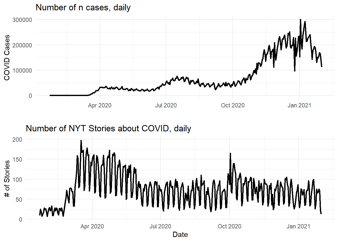 (Note: you may have gotten a warning or note that one row was removed. This is because the
 new_case variable from the data_covid dataset is NA for the date of January 22, 2021). You could remove this row before doing this analysis. I would not recommend using complete.cases() in this instance, though, because the death columns (total_deaths and new_deaths) don’t start until February 29, 2021.
7.4 Misc
7.4.1 Merging with an Index
As I mentioned previously, the data frames we used start/stop at different points.
head(data_nyt_count$date)## [1] "2020-01-08" "2020-01-09" "2020-01-10" "2020-01-11" "2020-01-15"
## [6] "2020-01-16"tail(data_nyt_count$date)## [1] "2021-01-26" "2021-01-27" "2021-01-28" "2021-01-29" "2021-01-30"
## [6] "2021-01-31"head(data_covid$date)## [1] "2020-01-22" "2020-01-23" "2020-01-24" "2020-01-25" "2020-01-26"
## [6] "2020-01-27"tail(data_covid$date)## [1] "2021-02-04" "2021-02-05" "2021-02-06" "2021-02-07" "2021-02-08"
## [6] "2021-02-09"Sometimes we want to clean the ends before merging them (or at least, I like to do this). If I’m working with multiple data frames, this is how I like to do it.
First, I’ll create an index:
data_index <- data.frame(date = seq.Date(as.Date("2020-01-23"), as.Date("2021-01-31"), by = "day"))Then, I use the index to merge all the additional data frames
full_data <- left_join(data_index, data_covid, by = "date") %>% left_join(data_nyt_count, by = "date")7.4.2 rbind
Sometimes, you want to “merge” by row rather than by column. In R, you can do this using the rbind() function (rbind stands for row bind). To do this, though, you need to have two data frames with the same number of columns. For example, imagine the covid dataset came in two parts:
data_covid_setA <- data_covid[1:200,]
data_covid_setB <- data_covid[201:385,]
How do you combine them? Using rbind()!
data_covid_fullset <- rbind(data_covid_setA, data_covid_setB)Note that this is the same number of rows as the original data_covid dataset!
7.4.3 Additional Resources
- “What if I want to combine more than two datasets?” I recommend the
reduce()function frompurrr(which is also atidyversepackage): https://stackoverflow.com/questions/8091303/simultaneously-merge-multiple-data-frames-in-a-list
- “I wanted to learn more about the
%in%operator!” That’s great! We’ll use it more once we get to the NLP section, but here’s a great tutorial on how to use in a general context: https://www.marsja.se/how-to-use-in-in-r/