13 Diabetic Monitoring

The following example will show-case one method processing data from strings and processing into dates and factors.

The folder Diabetes-Data is referenced from <https://archive.ics.uci.edu/ml/datasets/Diabetes>. as per the website:

Diabetes Data Set

Diabetes Data Set Download: Data Folder, Data Set Description

Abstract: This diabetes dataset is from AIM ’94

Characteristics of Diabetes Data Set on https://archive.ics.uci.edu/ml/datasets/Diabetes

Data Set Characteristics: Multivariate, Time-Series Number of Instances: ? Area: Life

Attribute Characteristics: Categorical, Integer Number of Attributes: 20 Date Donated Not Reported

Associated Tasks: Missing Values? ? Number of Web Hits:
561559

as reported on of April 2021

Source: Michael Kahn, MD, PhD, Washington University, St. Louis, MO

Characteristics of Diabetes Data Set on https://archive.ics.uci.edu/ml/datasets/Diabetes
Data Set Characteristics:	Multivariate, Time-Series	Number of Instances:	?	Area:	Life
Attribute Characteristics:	Categorical, Integer	Number of Attributes:	20	Date Donated	Not Reported
Associated Tasks:		Missing Values?	?	Number of Web Hits:	561559 as reported on of April 2021

Data Set Information: Diabetes patient records were obtained from two sources: an automatic electronic recording device and paper records. The automatic device had an internal clock to timestamp events, whereas the paper records only provided “logical time” slots (breakfast, lunch, dinner, bedtime). For paper records, fixed times were assigned to breakfast (08:00), lunch (12:00), dinner (18:00), and bedtime (22:00). Thus paper records have fictitious uniform recording times whereas electronic records have more realistic time stamps.

Diabetes files consist of four fields per record. Each field is separated by a tab and each record is separated by a newline.

File format:

Date in MM-DD-YYYY format

Time in XX:YY format

Code

Value

The Code field is deciphered as follows:

33 = Regular insulin dose

34 = NPH insulin dose

35 = UltraLente insulin dose

48 = Unspecified blood glucose measurement

57 = Unspecified blood glucose measurement

58 = Pre-breakfast blood glucose measurement

59 = Post-breakfast blood glucose measurement

60 = Pre-lunch blood glucose measurement

61 = Post-lunch blood glucose measurement

62 = Pre-supper blood glucose measurement

63 = Post-supper blood glucose measurement

64 = Pre-snack blood glucose measurement

65 = Hypoglycemic symptoms

66 = Typical meal ingestion

67 = More-than-usual meal ingestion

68 = Less-than-usual meal ingestion

69 = Typical exercise activity

70 = More-than-usual exercise activity

71 = Less-than-usual exercise activity

72 = Unspecified special event

\(~\)

13.1 Load Data

Week_6_wd <-  file.path('Week_6')
Week_6_DATA <- file.path(Week_6_wd,"DATA")
Week_6_Funs <- file.path(Week_6_wd,"FUNCTIONS")

DM2_DATA <- file.path(Week_6_wd,'Diabetes-Data')
DM2_DATA
#> [1] "Week_6/Diabetes-Data"

list_of_file_paths <- list.files(path = DM2_DATA,
                                 pattern = 'data-',
                                 recursive = TRUE,
                                 full.names = TRUE)
list_of_file_paths
#>  [1] "Week_6/Diabetes-Data/data-01" "Week_6/Diabetes-Data/data-02"
#>  [3] "Week_6/Diabetes-Data/data-03" "Week_6/Diabetes-Data/data-04"
#>  [5] "Week_6/Diabetes-Data/data-05" "Week_6/Diabetes-Data/data-06"
#>  [7] "Week_6/Diabetes-Data/data-07" "Week_6/Diabetes-Data/data-08"
#>  [9] "Week_6/Diabetes-Data/data-09" "Week_6/Diabetes-Data/data-10"
#> [11] "Week_6/Diabetes-Data/data-11" "Week_6/Diabetes-Data/data-12"
#> [13] "Week_6/Diabetes-Data/data-13" "Week_6/Diabetes-Data/data-14"
#> [15] "Week_6/Diabetes-Data/data-15" "Week_6/Diabetes-Data/data-16"
#> [17] "Week_6/Diabetes-Data/data-17" "Week_6/Diabetes-Data/data-18"
#> [19] "Week_6/Diabetes-Data/data-19" "Week_6/Diabetes-Data/data-20"
#> [21] "Week_6/Diabetes-Data/data-21" "Week_6/Diabetes-Data/data-22"
#> [23] "Week_6/Diabetes-Data/data-23" "Week_6/Diabetes-Data/data-24"
#> [25] "Week_6/Diabetes-Data/data-25" "Week_6/Diabetes-Data/data-26"
#> [27] "Week_6/Diabetes-Data/data-27" "Week_6/Diabetes-Data/data-28"
#> [29] "Week_6/Diabetes-Data/data-29" "Week_6/Diabetes-Data/data-30"
#> [31] "Week_6/Diabetes-Data/data-31" "Week_6/Diabetes-Data/data-32"
#> [33] "Week_6/Diabetes-Data/data-33" "Week_6/Diabetes-Data/data-34"
#> [35] "Week_6/Diabetes-Data/data-35" "Week_6/Diabetes-Data/data-36"
#> [37] "Week_6/Diabetes-Data/data-37" "Week_6/Diabetes-Data/data-38"
#> [39] "Week_6/Diabetes-Data/data-39" "Week_6/Diabetes-Data/data-40"
#> [41] "Week_6/Diabetes-Data/data-41" "Week_6/Diabetes-Data/data-42"
#> [43] "Week_6/Diabetes-Data/data-43" "Week_6/Diabetes-Data/data-44"
#> [45] "Week_6/Diabetes-Data/data-45" "Week_6/Diabetes-Data/data-46"
#> [47] "Week_6/Diabetes-Data/data-47" "Week_6/Diabetes-Data/data-48"
#> [49] "Week_6/Diabetes-Data/data-49" "Week_6/Diabetes-Data/data-50"
#> [51] "Week_6/Diabetes-Data/data-51" "Week_6/Diabetes-Data/data-52"
#> [53] "Week_6/Diabetes-Data/data-53" "Week_6/Diabetes-Data/data-54"
#> [55] "Week_6/Diabetes-Data/data-55" "Week_6/Diabetes-Data/data-56"
#> [57] "Week_6/Diabetes-Data/data-57" "Week_6/Diabetes-Data/data-58"
#> [59] "Week_6/Diabetes-Data/data-59" "Week_6/Diabetes-Data/data-60"
#> [61] "Week_6/Diabetes-Data/data-61" "Week_6/Diabetes-Data/data-62"
#> [63] "Week_6/Diabetes-Data/data-63" "Week_6/Diabetes-Data/data-64"
#> [65] "Week_6/Diabetes-Data/data-65" "Week_6/Diabetes-Data/data-66"
#> [67] "Week_6/Diabetes-Data/data-67" "Week_6/Diabetes-Data/data-68"
#> [69] "Week_6/Diabetes-Data/data-69" "Week_6/Diabetes-Data/data-70"

library('tidyverse')
#> ── Attaching packages ─────────────────────────────────────── tidyverse 1.3.2 ──
#> ✔ ggplot2 3.4.0      ✔ purrr   1.0.0 
#> ✔ tibble  3.1.8      ✔ dplyr   1.0.10
#> ✔ tidyr   1.2.1      ✔ stringr 1.5.0 
#> ✔ readr   2.1.3      ✔ forcats 0.5.2 
#> ── Conflicts ────────────────────────────────────────── tidyverse_conflicts() ──
#> ✖ dplyr::filter() masks stats::filter()
#> ✖ dplyr::lag()    masks stats::lag()

tibble_of_file_paths <- tibble(list_of_file_paths) %>%
   mutate(full_path = list_of_file_paths) %>%
   mutate(file_no = str_replace(string = full_path,
                            pattern = paste0(DM2_DATA,'/data-'),
                            replacement = '')) 

tibble_of_file_paths
#> # A tibble: 70 × 3
#>   list_of_file_paths           full_path                    file_no
#>   <chr>                        <chr>                        <chr>  
#> 1 Week_6/Diabetes-Data/data-01 Week_6/Diabetes-Data/data-01 01     
#> 2 Week_6/Diabetes-Data/data-02 Week_6/Diabetes-Data/data-02 02     
#> 3 Week_6/Diabetes-Data/data-03 Week_6/Diabetes-Data/data-03 03     
#> 4 Week_6/Diabetes-Data/data-04 Week_6/Diabetes-Data/data-04 04     
#> 5 Week_6/Diabetes-Data/data-05 Week_6/Diabetes-Data/data-05 05     
#> 6 Week_6/Diabetes-Data/data-06 Week_6/Diabetes-Data/data-06 06     
#> # … with 64 more rows

read_in_text_from_file_no <- function(my_file_no){

  enquo_by <- enquo(my_file_no)

  cur_file <- tibble_of_file_paths %>%
    filter(file_no == !!enquo_by)

  cur_path <- as.character(cur_file$full_path)

   dat <- readr::read_tsv(cur_path,
                           col_names = c('Date',"Time","Code","Value"),
                           col_types = cols(col_character(), col_character(), col_character(), col_character())
                           ) %>%
      mutate(file_no = as.numeric(cur_file$file_no))

   return(dat)
}

library('furrr')
#> Loading required package: future
no_cores <- availableCores() - 1
no_cores
#> system 
#>     15

future::plan(multicore, workers = no_cores)

DM2_TIME_RAW <- furrr::future_map_dfr(tibble_of_file_paths$file_no, # list of columns 
                      function(x){ read_in_text_from_file_no(x) })

DM2_TIME_RAW %>%
  saveRDS('DATA/DM2_TIME_RAW.RDS')

DM2_TIME_RAW <- readRDS('DATA/DM2_TIME_RAW.RDS')

\(~\)

13.2 Decode Table

Code_Table <- tribble(
  ~ Code, ~ Code_Description,
  33 , "Regular insulin dose",
  34 , "NPH insulin dose",
  35 , "UltraLente insulin dose",
  48 , "Unspecified blood glucose measurement", # This decode value is the same as 57
  57 , "Unspecified blood glucose measurement", # This decode value is the same as 48
  58 , "Pre-breakfast blood glucose measurement",
  59 , "Post-breakfast blood glucose measurement",
  60 , "Pre-lunch blood glucose measurement",
  61 , "Post-lunch blood glucose measurement",
  62 , "Pre-supper blood glucose measurement",
  63 , "Post-supper blood glucose measurement",
  64 , "Pre-snack blood glucose measurement",
  65 , "Hypoglycemic symptoms",
  66 , "Typical meal ingestion",
  67 , "More-than-usual meal ingestion",
  68 , "Less-than-usual meal ingestion",
  69 , "Typical exercise activity",
  70 , "More-than-usual exercise activity",
  71 , "Less-than-usual exercise activity",
  72 , "Unspecified special event") %>% # What does this mean? 
  mutate(Code_Invalid = if_else(Code %in% c(48,57,72), TRUE, FALSE)) %>%
  mutate(Code_New = if_else(Code_Invalid == TRUE, 999, Code)) 

Code_Table
#> # A tibble: 20 × 4
#>    Code Code_Description                        Code_Invalid Code_New
#>   <dbl> <chr>                                   <lgl>           <dbl>
#> 1    33 Regular insulin dose                    FALSE              33
#> 2    34 NPH insulin dose                        FALSE              34
#> 3    35 UltraLente insulin dose                 FALSE              35
#> 4    48 Unspecified blood glucose measurement   TRUE              999
#> 5    57 Unspecified blood glucose measurement   TRUE              999
#> 6    58 Pre-breakfast blood glucose measurement FALSE              58
#> # … with 14 more rows

Code_Table_Factor <- Code_Table %>%
  filter(Code_Invalid == FALSE) %>%
  mutate(Code_Factor = factor(paste0("C_",Code_New)))

Code_Table_Factor
#> # A tibble: 17 × 5
#>    Code Code_Description                         Code_Invalid Code_New Code_Fa…¹
#>   <dbl> <chr>                                    <lgl>           <dbl> <fct>    
#> 1    33 Regular insulin dose                     FALSE              33 C_33     
#> 2    34 NPH insulin dose                         FALSE              34 C_34     
#> 3    35 UltraLente insulin dose                  FALSE              35 C_35     
#> 4    58 Pre-breakfast blood glucose measurement  FALSE              58 C_58     
#> 5    59 Post-breakfast blood glucose measurement FALSE              59 C_59     
#> 6    60 Pre-lunch blood glucose measurement      FALSE              60 C_60     
#> # … with 11 more rows, and abbreviated variable name ¹Code_Factor

13.3 Format Data

library('lubridate')
#> Loading required package: timechange
#> 
#> Attaching package: 'lubridate'
#> The following objects are masked from 'package:base':
#> 
#>     date, intersect, setdiff, union

DM2_TIME <- DM2_TIME_RAW %>%
  mutate(Date_Time_Char = paste0(Date, ' ', Time)) %>%
  mutate(Date_Time = mdy_hm(Date_Time_Char))  %>%
  mutate(Value_Num = as.numeric(Value)) %>%
  mutate(Code = as.numeric(Code)) %>%
  mutate(Record_ID = row_number())
#> Warning: 45 failed to parse.
#> Warning in mask$eval_all_mutate(quo): NAs introduced by coercion
  
DM2_TIME
#> # A tibble: 29,330 × 9
#>   Date     Time   Code Value file_no Date_…¹ Date_Time           Value…² Recor…³
#>   <chr>    <chr> <dbl> <chr>   <dbl> <chr>   <dttm>                <dbl>   <int>
#> 1 04-21-1… 9:09     58 100         1 04-21-… 1991-04-21 09:09:00     100       1
#> 2 04-21-1… 9:09     33 009         1 04-21-… 1991-04-21 09:09:00       9       2
#> 3 04-21-1… 9:09     34 013         1 04-21-… 1991-04-21 09:09:00      13       3
#> 4 04-21-1… 17:08    62 119         1 04-21-… 1991-04-21 17:08:00     119       4
#> 5 04-21-1… 17:08    33 007         1 04-21-… 1991-04-21 17:08:00       7       5
#> 6 04-21-1… 22:51    48 123         1 04-21-… 1991-04-21 22:51:00     123       6
#> # … with 29,324 more rows, and abbreviated variable names ¹Date_Time_Char,
#> #   ²Value_Num, ³Record_ID

UnKnown_Measurements <- DM2_TIME %>%
  left_join(Code_Table_Factor, by='Code') %>%
  filter(is.na(Code_Description) | is.na(Date_Time) | is.na(Value_Num) | Code_Invalid == TRUE | Code_New == 999 )

UnKnown_Measurements
#> # A tibble: 3,171 × 13
#>   Date     Time   Code Value file_no Date_…¹ Date_Time           Value…² Recor…³
#>   <chr>    <chr> <dbl> <chr>   <dbl> <chr>   <dttm>                <dbl>   <int>
#> 1 04-21-1… 22:51    48 123         1 04-21-… 1991-04-21 22:51:00     123       6
#> 2 04-24-1… 22:09    48 340         1 04-24-… 1991-04-24 22:09:00     340      23
#> 3 04-25-1… 21:54    48 288         1 04-25-… 1991-04-25 21:54:00     288      31
#> 4 04-28-1… 22:30    48 200         1 04-28-… 1991-04-28 22:30:00     200      49
#> 5 04-29-1… 22:28    48 081         1 04-29-… 1991-04-29 22:28:00      81      58
#> 6 04-30-1… 23:06    48 104         1 04-30-… 1991-04-30 23:06:00     104      67
#> # … with 3,165 more rows, 4 more variables: Code_Description <chr>,
#> #   Code_Invalid <lgl>, Code_New <dbl>, Code_Factor <fct>, and abbreviated
#> #   variable names ¹Date_Time_Char, ²Value_Num, ³Record_ID

Known_Measurements <- DM2_TIME %>%
  anti_join(UnKnown_Measurements %>% select(Record_ID)) %>%
  left_join(Code_Table_Factor, by='Code')
#> Joining, by = "Record_ID"

Known_Measurements
#> # A tibble: 26,159 × 13
#>   Date     Time   Code Value file_no Date_…¹ Date_Time           Value…² Recor…³
#>   <chr>    <chr> <dbl> <chr>   <dbl> <chr>   <dttm>                <dbl>   <int>
#> 1 04-21-1… 9:09     58 100         1 04-21-… 1991-04-21 09:09:00     100       1
#> 2 04-21-1… 9:09     33 009         1 04-21-… 1991-04-21 09:09:00       9       2
#> 3 04-21-1… 9:09     34 013         1 04-21-… 1991-04-21 09:09:00      13       3
#> 4 04-21-1… 17:08    62 119         1 04-21-… 1991-04-21 17:08:00     119       4
#> 5 04-21-1… 17:08    33 007         1 04-21-… 1991-04-21 17:08:00       7       5
#> 6 04-22-1… 7:35     58 216         1 04-22-… 1991-04-22 07:35:00     216       7
#> # … with 26,153 more rows, 4 more variables: Code_Description <chr>,
#> #   Code_Invalid <lgl>, Code_New <dbl>, Code_Factor <fct>, and abbreviated
#> #   variable names ¹Date_Time_Char, ²Value_Num, ³Record_ID

\(~\)

13.4 View Data

Known_Measurements %>%
  ggplot(aes(x=Date_Time, y=Value_Num, color=Code_Factor)) +
  geom_point()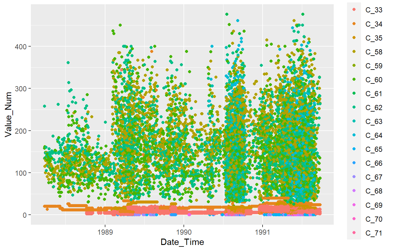

Features_Percent_Complete <- function(data, Percent_Complete = 0){
  
  SumNa <- function(col){sum(is.na(col))}
  
  na_sums <- data %>% 
    summarise_all(SumNa) %>%
    tidyr::pivot_longer(everything() ,names_to = 'feature', values_to = 'SumNa') %>%
    arrange(-SumNa) %>%
    mutate(PctNa = SumNa/nrow(data)) %>%
    mutate(PctComp = (1 - PctNa)*100)
  
  data_out <- na_sums %>%
    filter(PctComp >= Percent_Complete)
  
return(data_out)
}

Feature_Percent_Complete_Graph <- function(data, Percent_Complete = 0 ){
  table <- Features_Percent_Complete(data, Percent_Complete)
  
  plot1 <- table %>%
    ggplot(aes(x=reorder(feature, PctComp), y =PctComp, fill=feature)) +
    geom_bar(stat = "identity") +
    coord_flip() +
    theme(legend.position = "none")
  return(plot1)
}

Feature_Percent_Complete_Graph(data = Known_Measurements %>% select(Date_Time, Value_Num, Code_Factor) )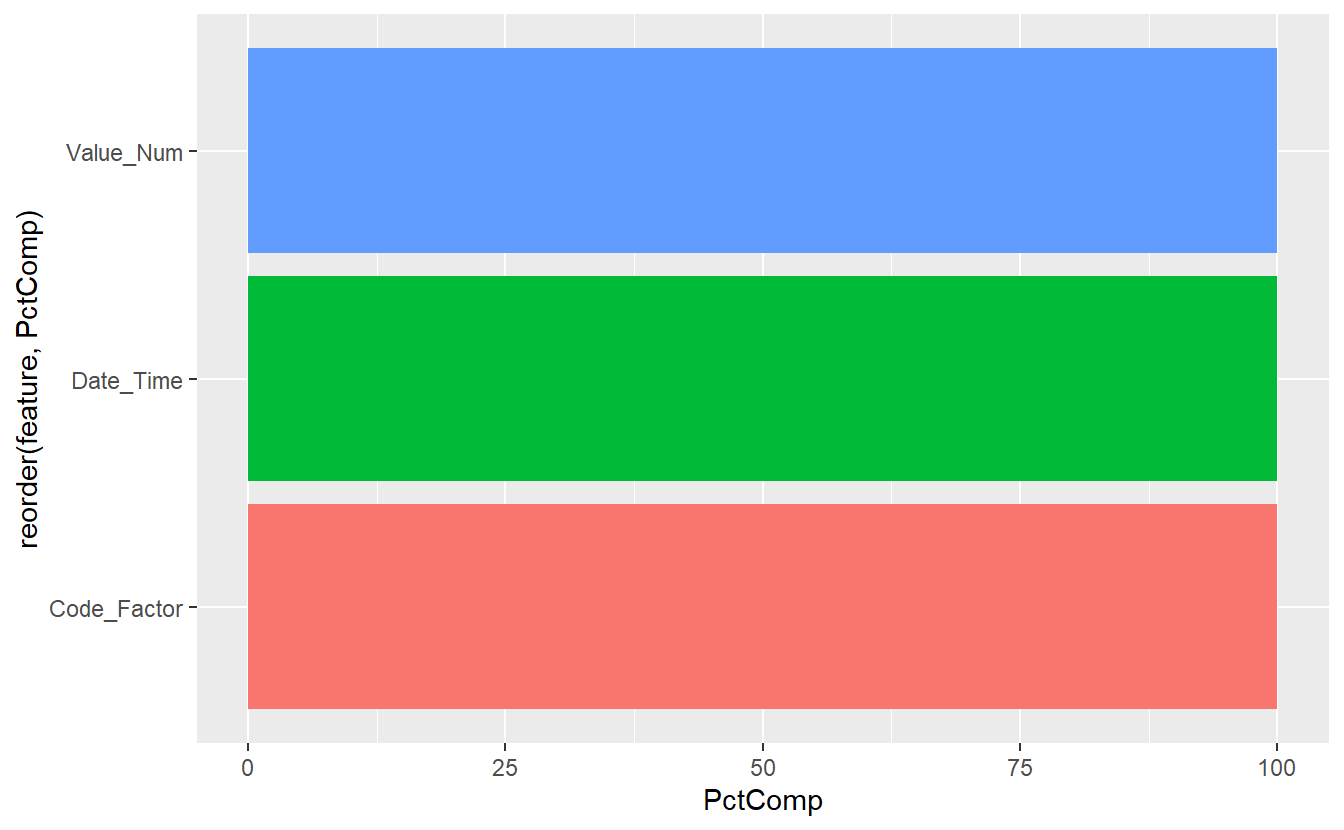

(#fig:5-percent-complete-graph-1 )Known Measurements Feature % Complete Graph

\(~\)

13.5 UnKnown Measurements

UnKnown_Measurements %>%
  ggplot(aes(x=Date_Time, y=Value_Num)) +
  geom_point() 
#> Warning: Removed 86 rows containing missing values (`geom_point()`).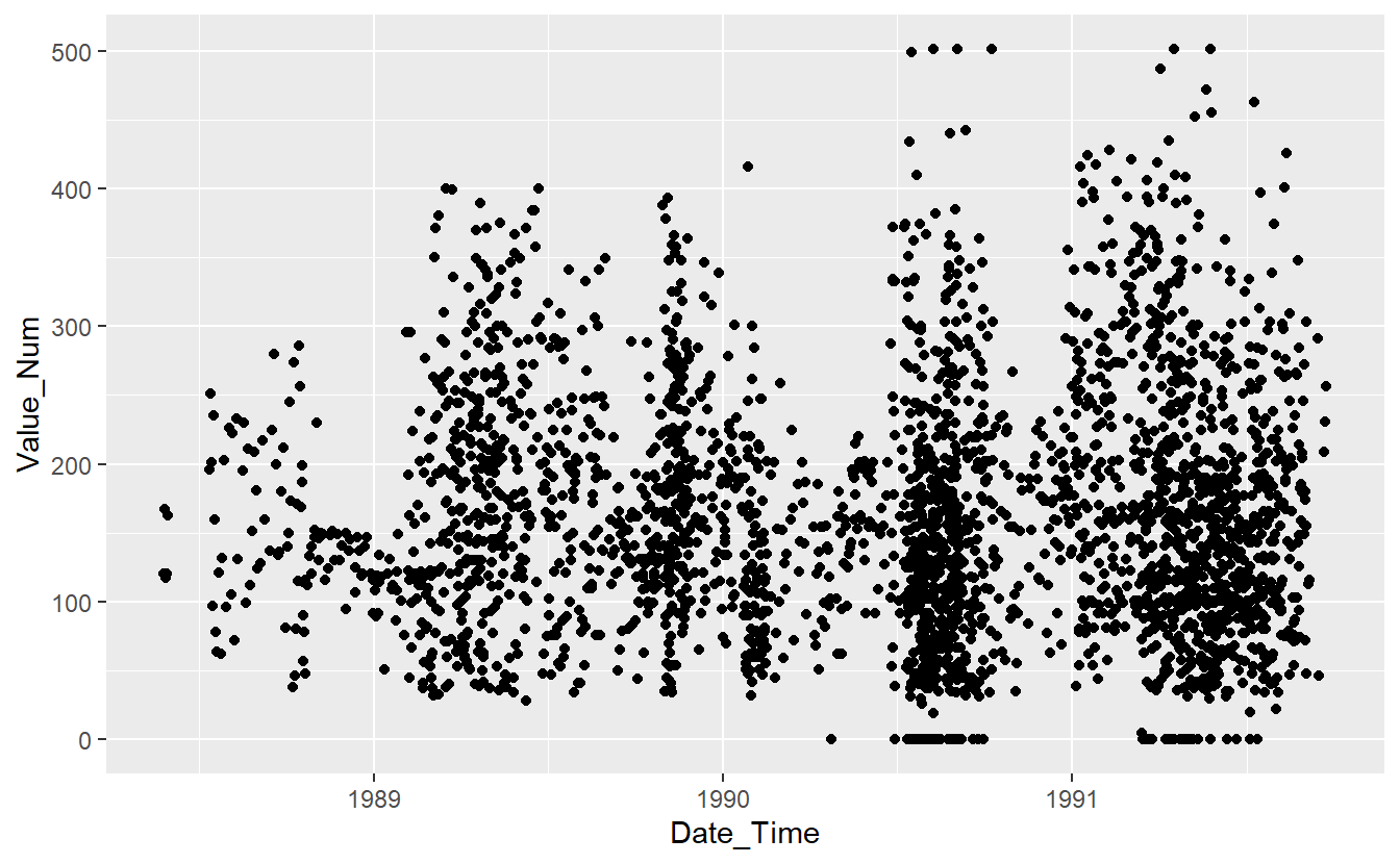

(#fig:5-unknown-fig-1 )UnKnown Measurements

\(~\)

13.6 Split Training Data

set.seed(123)
train_records <- sample(Known_Measurements$Record_ID, 
                      size = nrow(Known_Measurements)*.6, 
                      replace = FALSE)


DATA.train <- Known_Measurements %>%
  filter(Record_ID %in% train_records)

DATA.test <- Known_Measurements %>%
  filter(!(Record_ID %in% train_records))

DATA.train %>% 
  ggplot(aes(x=Date_Time, y=Value_Num, color=Code_Factor)) +
  geom_point()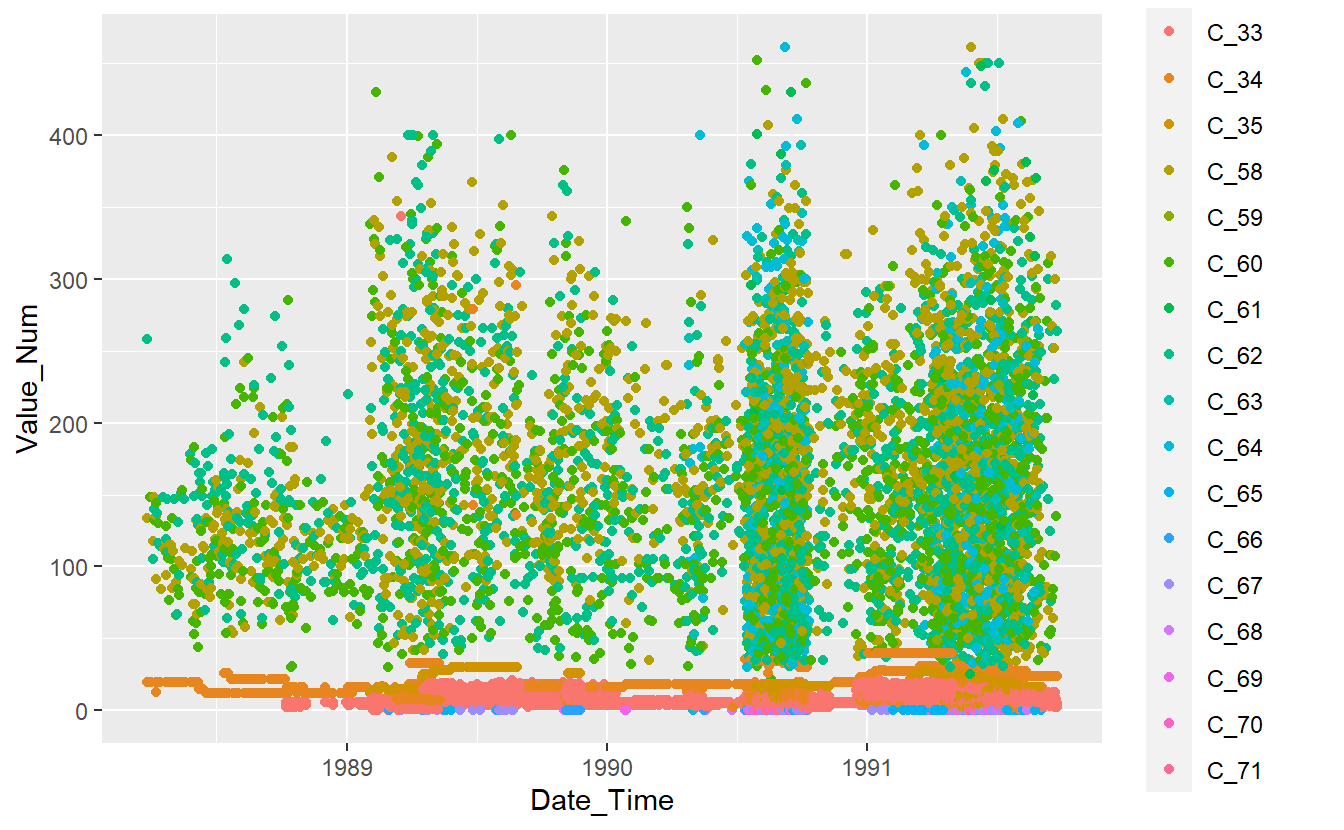

Figure 13.1: Plot of Training Data

DATA.test %>% 
  ggplot(aes(x=Date_Time, y=Value_Num, color=Code_Factor)) +
  geom_point()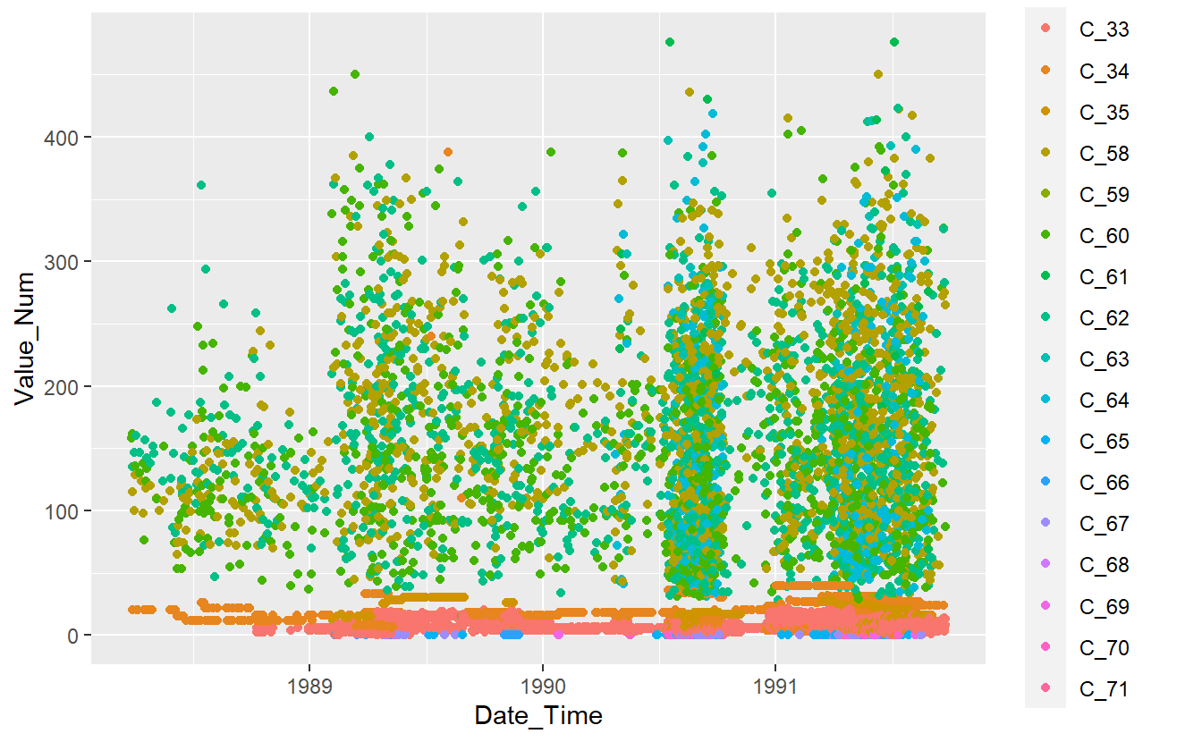

Figure 13.2: Plot of Test Data

\(~\)

13.7 Fit a Model

library('randomForest')
#> randomForest 4.7-1.1
#> Type rfNews() to see new features/changes/bug fixes.
#> 
#> Attaching package: 'randomForest'
#> The following object is masked from 'package:dplyr':
#> 
#>     combine
#> The following object is masked from 'package:ggplot2':
#> 
#>     margin

rf_model <- randomForest(Code_Factor ~ Date_Time + Value_Num,
                         data = DATA.train,
                         ntree = 659,
                         importance = TRUE)

13.7.1 Random Forest Ouput

Here’s the output of Random Forest

rf_model
#> 
#> Call:
#>  randomForest(formula = Code_Factor ~ Date_Time + Value_Num, data = DATA.train,      ntree = 659, importance = TRUE) 
#>                Type of random forest: classification
#>                      Number of trees: 659
#> No. of variables tried at each split: 1
#> 
#>         OOB estimate of  error rate: 36.11%
#> Confusion matrix:
#>      C_33 C_34 C_35 C_58 C_59 C_60 C_61 C_62 C_63 C_64 C_65 C_66 C_67 C_68 C_69
#> C_33 5377  231   59    0    0    0    0    2    0    0    1    1    3    0    0
#> C_34  669 1586   59    4    0    2    0    1    0    0    0    0    0    0    0
#> C_35  167   88  398    0    0    0    0    0    0    0    0    0    0    0    0
#> C_58    0    5    3  969    1  473    6  551   21   79    0    0    0    0    0
#> C_59    0    0    0    3    0    3    0    5    0    0    0    0    0    0    0
#> C_60    0   10    1  555    2  534    1  465    9   66    0    0    0    0    0
#> C_61    0    0    1   12    0    7    4   12    0    4    0    0    0    0    0
#> C_62    0    8    0  651    2  440    1  680   10   85    0    0    0    0    0
#> C_63    0    0    0   45    0   25    0   35   26    5    0    0    0    0    0
#> C_64    0    5    0  137    0   85    0  127    7  173    0    1    0    0    0
#> C_65    0    0    0    0    0    0    0    0    0    0   47    4  143    0    0
#> C_66    1    0    0    0    0    0    0    0    0    0    3   66   27    0    0
#> C_67    1    0    0    0    0    0    0    0    0    0   32    1  167    0    0
#> C_68    0    0    0    0    0    0    0    0    0    0    3    2   16    0    0
#> C_69    0    0    0    0    0    0    0    0    0    0    3   11   25    0    0
#> C_70    0    0    0    0    0    0    0    0    0    0    4    1   85    0    0
#> C_71    0    0    0    0    0    0    0    0    0    0    8    0   47    0    0
#>      C_70 C_71 class.error
#> C_33    0    0  0.05234403
#> C_34    0    0  0.31667385
#> C_35    0    0  0.39050536
#> C_58    0    0  0.54032258
#> C_59    0    0  1.00000000
#> C_60    0    0  0.67498478
#> C_61    0    0  0.90000000
#> C_62    0    0  0.63771977
#> C_63    0    0  0.80882353
#> C_64    0    0  0.67663551
#> C_65    0    0  0.75773196
#> C_66    0    0  0.31958763
#> C_67    0    0  0.16915423
#> C_68    0    0  1.00000000
#> C_69    0    0  1.00000000
#> C_70    0    0  1.00000000
#> C_71    0    0  1.00000000

The Confusion Matrix that we see above is the confusion matrix from fitting the model against the training data so it is overly optimistic in terms of predictions.

Random Forest is a collection of Decision Trees, we can look at the individual trees in the forest by using one of the two following functions.

library(ggraph)
library(igraph)
#> 
#> Attaching package: 'igraph'
#> The following objects are masked from 'package:lubridate':
#> 
#>     %--%, union
#> The following objects are masked from 'package:future':
#> 
#>     %->%, %<-%
#> The following objects are masked from 'package:dplyr':
#> 
#>     as_data_frame, groups, union
#> The following objects are masked from 'package:purrr':
#> 
#>     compose, simplify
#> The following object is masked from 'package:tidyr':
#> 
#>     crossing
#> The following object is masked from 'package:tibble':
#> 
#>     as_data_frame
#> The following objects are masked from 'package:stats':
#> 
#>     decompose, spectrum
#> The following object is masked from 'package:base':
#> 
#>     union

plot_rf_tree <- function(final_model, tree_num, shorten_label = TRUE) {
  # get tree by index
  tree <- randomForest::getTree(final_model, 
                                k = tree_num, 
                                labelVar = TRUE) %>%
    tibble::rownames_to_column() %>%
    # make leaf split points to NA, so the 0s won't get plotted
    mutate(`split point` = ifelse(is.na(prediction), `split point`, NA))
  
  # prepare data frame for graph
  graph_frame <- data.frame(from = rep(tree$rowname, 2),
                            to = c(tree$`left daughter`, tree$`right daughter`))
  
  # convert to graph and delete the last node that we don't want to plot
  graph <- graph_from_data_frame(graph_frame) %>%
    delete_vertices("0")
  
  # set node labels
  V(graph)$node_label <- gsub("_", " ", as.character(tree$`split var`))
  
  if (shorten_label) {
    V(graph)$leaf_label <- substr(as.character(tree$prediction), 1, 1)
    }
  
  V(graph)$split <- as.character(round(tree$`split point`, digits = 2))
  
  # plot
  plot <- ggraph(graph, 'tree') + 
    theme_graph() +
    geom_edge_link() +
    geom_node_point() +
    geom_node_label(aes(label = leaf_label, fill = leaf_label), na.rm = TRUE, 
                    repel = FALSE, colour = "white",
                    show.legend = FALSE)
  
  print(plot)
}

plot_rf_tree(rf_model, 456)
#> Warning: Duplicated aesthetics after name standardisation: na.rm
#> Warning: Using the `size` aesthetic in this geom was deprecated in ggplot2 3.4.0.
#> ℹ Please use `linewidth` in the `default_aes` field and elsewhere instead.
#> Warning: Removed 2855 rows containing missing values (`geom_label()`).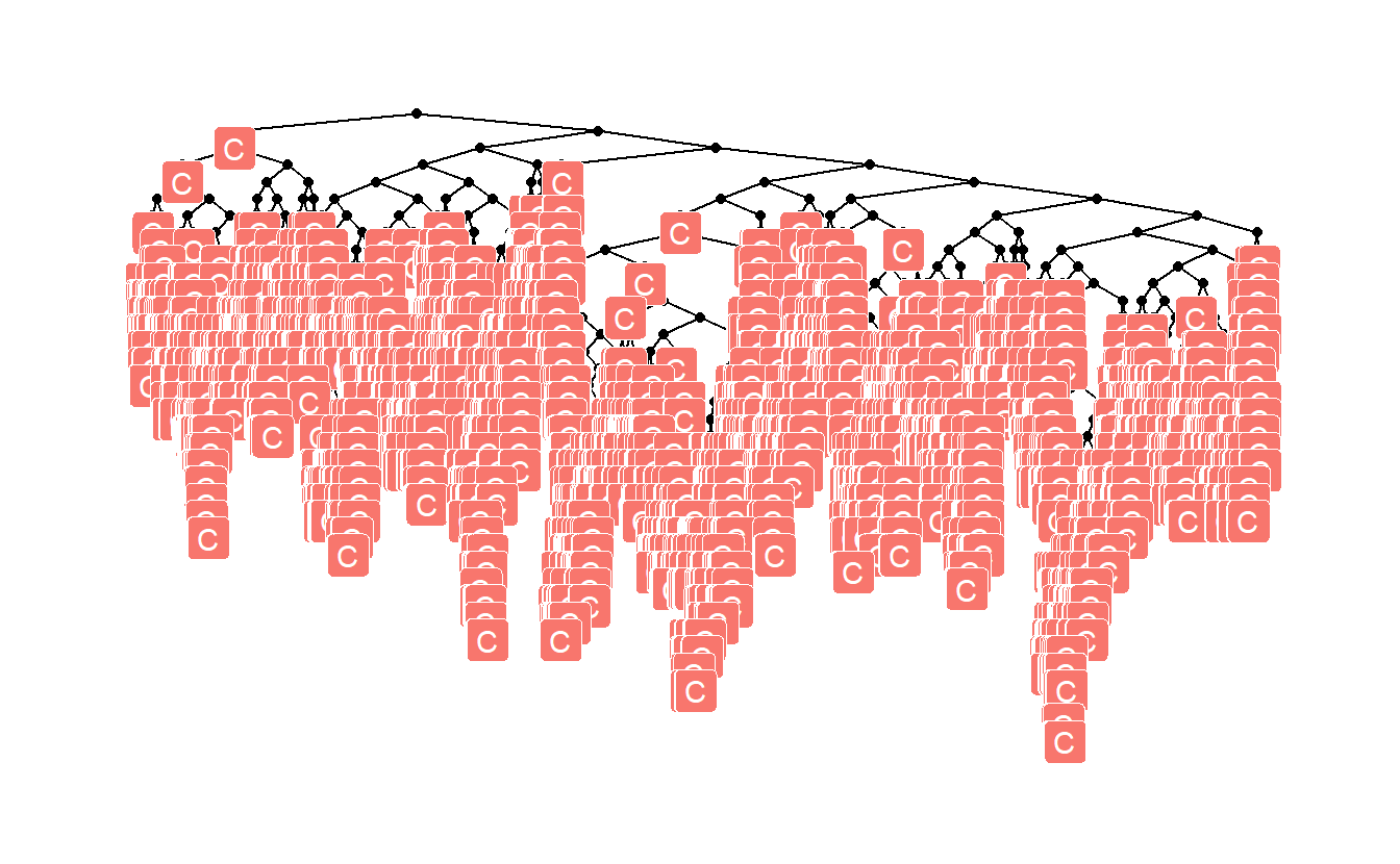

Random Forest models normally come equipped with feature importances:

varImpPlot(rf_model)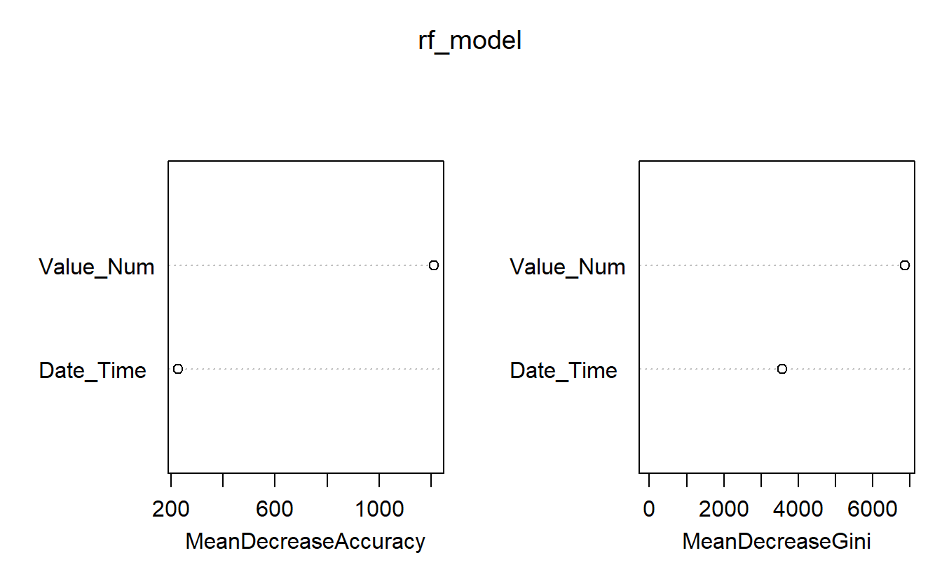

Figure 13.3: Feature Importances of Base Model

For instance, above we see that Date_Time is more in terms classifying the measurement as opposed to Value_Num

We can also extract the feature importances for each of the classes:

caret::varImp(rf_model, scale = FALSE) %>% 
  t() %>%  # transpose the entire dataframe
  as_tibble(rownames = 'Class' ) # turn it back to a tibble
#> # A tibble: 17 × 3
#>   Class Date_Time Value_Num
#>   <chr>     <dbl>     <dbl>
#> 1 C_33   0.0969     0.517  
#> 2 C_34   0.264      0.509  
#> 3 C_35   0.373      0.507  
#> 4 C_58   0.0481     0.246  
#> 5 C_59  -0.000723  -0.00106
#> 6 C_60   0.0413     0.194  
#> # … with 11 more rows

The Random Forest model also has a plot associated with it:

plot(rf_model)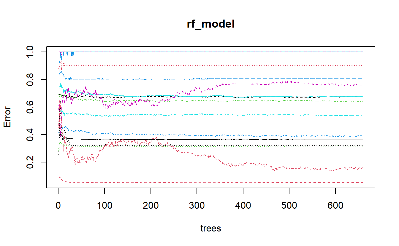

Figure 13.4: plot of randomForest model output

Let’s see if we can figure out what is going on with the above graph. We can extract the err.rate and ntree from the model object and place them in a matplot to match the above graph.

err <- rf_model$err.rate

N_trees <- 1:rf_model$ntree

matplot(N_trees , err, type = 'l', xlab="trees", ylab="Error")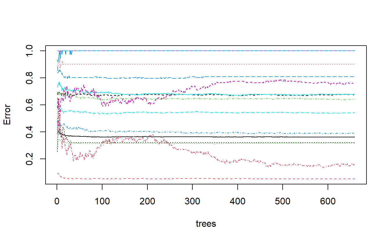

Figure 13.5: derivation of plot of randomForest model output

We can improve this a bit by performing the computations ourselves and keeping track of things:

err2 <- as_tibble(err, rownames='n_trees')

err2 %>%
  glimpse()
#> Rows: 659
#> Columns: 19
#> $ n_trees <chr> "1", "2", "3", "4", "5", "6", "7", "8", "9", "10", "11", "12",…
#> $ OOB     <dbl> 0.3888985, 0.4010195, 0.4031778, 0.4038520, 0.3991778, 0.39185…
#> $ C_33    <dbl> 0.09125475, 0.09435626, 0.08716876, 0.08636837, 0.08526068, 0.…
#> $ C_34    <dbl> 0.2818713, 0.3272194, 0.3405500, 0.3448990, 0.3397964, 0.33502…
#> $ C_35    <dbl> 0.4140625, 0.4623116, 0.4863732, 0.4646840, 0.4636678, 0.45928…
#> $ C_58    <dbl> 0.6084724, 0.6100235, 0.6091371, 0.5932394, 0.5891270, 0.58295…
#> $ C_59    <dbl> 1, 1, 1, 1, 1, 1, 1, 1, 1, 1, 1, 1, 1, 1, 1, 1, 1, 1, 1, 1, 1,…
#> $ C_60    <dbl> 0.6745363, 0.6883768, 0.7014563, 0.6958763, 0.6922034, 0.68802…
#> $ C_61    <dbl> 0.8823529, 0.8695652, 0.9062500, 0.9166667, 0.9166667, 0.94444…
#> $ C_62    <dbl> 0.6921986, 0.6770186, 0.6747851, 0.6957352, 0.6849882, 0.67257…
#> $ C_63    <dbl> 0.8837209, 0.8354430, 0.8446602, 0.8547009, 0.8412698, 0.85937…
#> $ C_64    <dbl> 0.7313433, 0.7507692, 0.7500000, 0.7707424, 0.7479508, 0.76247…
#> $ C_65    <dbl> 0.5774648, 0.6504065, 0.4697987, 0.4756098, 0.3815029, 0.47777…
#> $ C_66    <dbl> 0.2564103, 0.3000000, 0.5769231, 0.6470588, 0.5617978, 0.48351…
#> $ C_67    <dbl> 0.5000000, 0.3931624, 0.6466667, 0.6190476, 0.6032609, 0.53968…
#> $ C_68    <dbl> 1, 1, 1, 1, 1, 1, 1, 1, 1, 1, 1, 1, 1, 1, 1, 1, 1, 1, 1, 1, 1,…
#> $ C_69    <dbl> 0.9333333, 0.9166667, 0.9354839, 0.9696970, 1.0000000, 0.97142…
#> $ C_70    <dbl> 1, 1, 1, 1, 1, 1, 1, 1, 1, 1, 1, 1, 1, 1, 1, 1, 1, 1, 1, 1, 1,…
#> $ C_71    <dbl> 1.0000000, 1.0000000, 1.0000000, 1.0000000, 1.0000000, 0.98076…


predicted_levels <- colnames(err2)[!colnames(err2) %in% c('n_trees','OOB')]
predicted_levels
#>  [1] "C_33" "C_34" "C_35" "C_58" "C_59" "C_60" "C_61" "C_62" "C_63" "C_64"
#> [11] "C_65" "C_66" "C_67" "C_68" "C_69" "C_70" "C_71"

plot <- err2 %>%
  select(-OOB) %>%
  pivot_longer(all_of(predicted_levels), names_to = "Class", values_to = "Error") %>%
  mutate(N_Trees = as.numeric(n_trees)) %>%
  ggplot(aes(x=N_Trees, y=Error, color=Class)) +
  geom_point() +
  geom_smooth(method = lm, formula = y ~ splines::bs(x, 3), se = FALSE) 
  
plot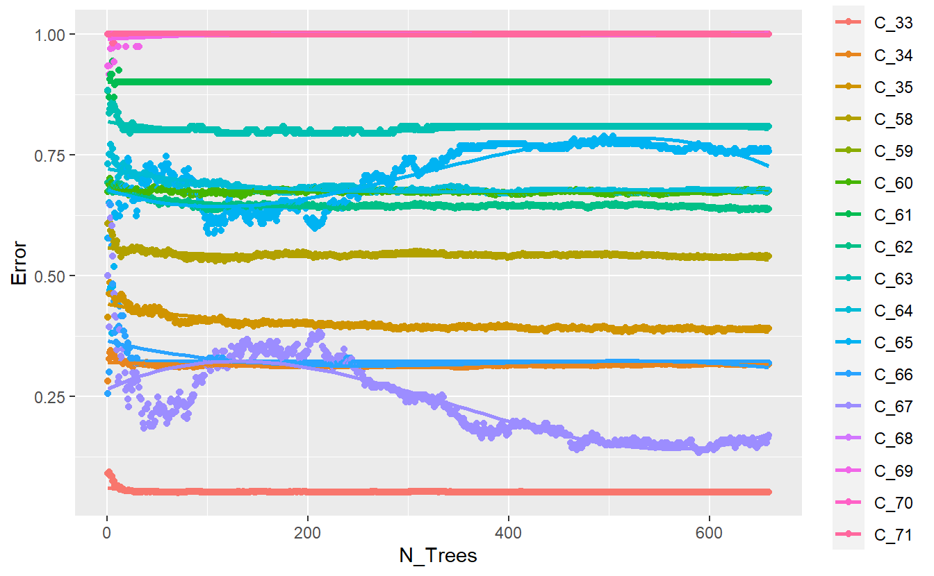

Figure 13.6: Improved plot of base randomForest model output

better_rand_forest_errors <- function(rf_model_obj){
  err <- rf_model_obj$err.rate
  
  err2 <- as_tibble(err, rownames='n_trees')
  
  predicted_levels <- colnames(err2)[!colnames(err2) %in% c('n_trees','OOB')]
  
  plot <- err2 %>%
  select(-OOB) %>%
  pivot_longer(all_of(predicted_levels), names_to = "Class", values_to = "Error") %>%
  mutate(N_Trees = as.numeric(n_trees)) %>%
  ggplot(aes(x=N_Trees, y=Error, color=Class)) +
  geom_point() +
  geom_smooth(method = lm, formula = y ~ splines::bs(x, 3), se = FALSE) 
  
  return(plot)
}

\(~\)

13.8 Evaluate Model Performace

DATA.test.Scored <- DATA.test %>%
  mutate(model = 'base')

First, we will get the expected classes for the test data:

DATA.test.Scored$pred <- predict(rf_model, DATA.test , 'response')

DATA.test.Scored %>%
  glimpse()
#> Rows: 10,464
#> Columns: 15
#> $ Date             <chr> "04-21-1991", "04-21-1991", "04-22-1991", "04-22-1991…
#> $ Time             <chr> "9:09", "9:09", "7:35", "7:35", "7:25", "7:29", "7:29…
#> $ Code             <dbl> 58, 34, 58, 34, 58, 58, 33, 34, 33, 62, 33, 62, 33, 3…
#> $ Value            <chr> "100", "013", "216", "013", "257", "067", "009", "014…
#> $ file_no          <dbl> 1, 1, 1, 1, 1, 1, 1, 1, 1, 1, 1, 1, 1, 1, 1, 1, 1, 1,…
#> $ Date_Time_Char   <chr> "04-21-1991 9:09", "04-21-1991 9:09", "04-22-1991 7:3…
#> $ Date_Time        <dttm> 1991-04-21 09:09:00, 1991-04-21 09:09:00, 1991-04-22…
#> $ Value_Num        <dbl> 100, 13, 216, 13, 257, 67, 9, 14, 2, 228, 7, 256, 8, …
#> $ Record_ID        <int> 1, 3, 7, 9, 13, 25, 26, 27, 32, 37, 38, 42, 43, 45, 5…
#> $ Code_Description <chr> "Pre-breakfast blood glucose measurement", "NPH insul…
#> $ Code_Invalid     <lgl> FALSE, FALSE, FALSE, FALSE, FALSE, FALSE, FALSE, FALS…
#> $ Code_New         <dbl> 58, 34, 58, 34, 58, 58, 33, 34, 33, 62, 33, 62, 33, 3…
#> $ Code_Factor      <fct> C_58, C_34, C_58, C_34, C_58, C_58, C_33, C_34, C_33,…
#> $ model            <chr> "base", "base", "base", "base", "base", "base", "base…
#> $ pred             <fct> C_60, C_35, C_58, C_35, C_62, C_63, C_33, C_33, C_33,…

library('yardstick')
#> For binary classification, the first factor level is assumed to be the event.
#> Use the argument `event_level = "second"` to alter this as needed.
#> 
#> Attaching package: 'yardstick'
#> The following object is masked from 'package:readr':
#> 
#>     spec
conf_mat.DATA.test.Scored <- conf_mat(DATA.test.Scored, 
                                      truth = Code_Factor, pred)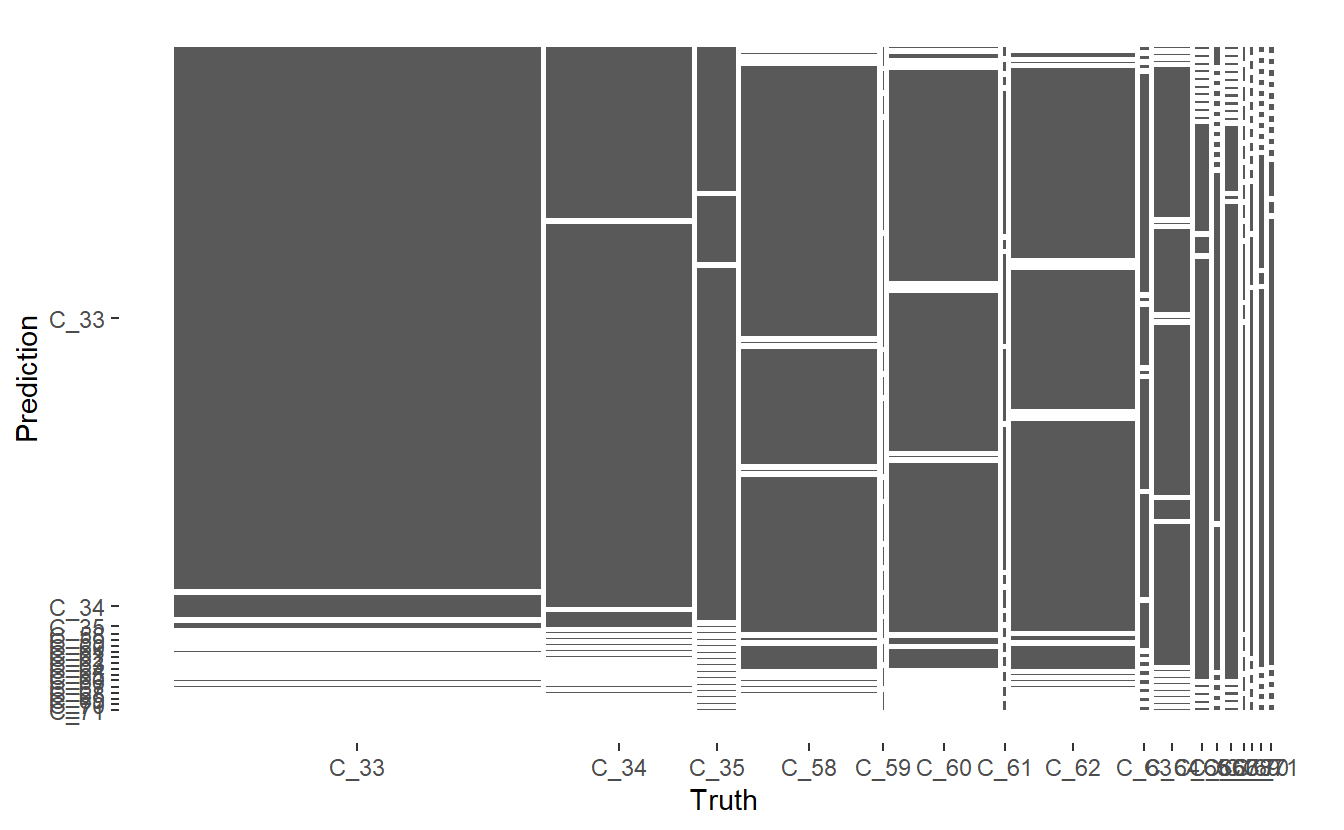

conf_mat.DATA.test.Scored %>%
  autoplot('mosaic')

Figure 13.7: Mosaic Confusion Matrix of Base Model

DATA.test.Scored %>%
  conf_mat(truth= Code_Factor, pred) %>%
  summary() %>%
  ggplot(aes(x=.metric, y=.estimate, fill= .metric)) +
  geom_bar(stat='identity', position = 'dodge') +
  coord_flip()
#> Warning: While computing multiclass `precision()`, some levels had no predicted events (i.e. `true_positive + false_positive = 0`). 
#> Precision is undefined in this case, and those levels will be removed from the averaged result.
#> Note that the following number of true events actually occured for each problematic event level:
#> 'C_68': 13
#> 'C_69': 29
#> 'C_70': 49
#> 'C_71': 43
#> While computing multiclass `precision()`, some levels had no predicted events (i.e. `true_positive + false_positive = 0`). 
#> Precision is undefined in this case, and those levels will be removed from the averaged result.
#> Note that the following number of true events actually occured for each problematic event level:
#> 'C_68': 13
#> 'C_69': 29
#> 'C_70': 49
#> 'C_71': 43
#> Warning: Removed 1 rows containing missing values (`geom_bar()`).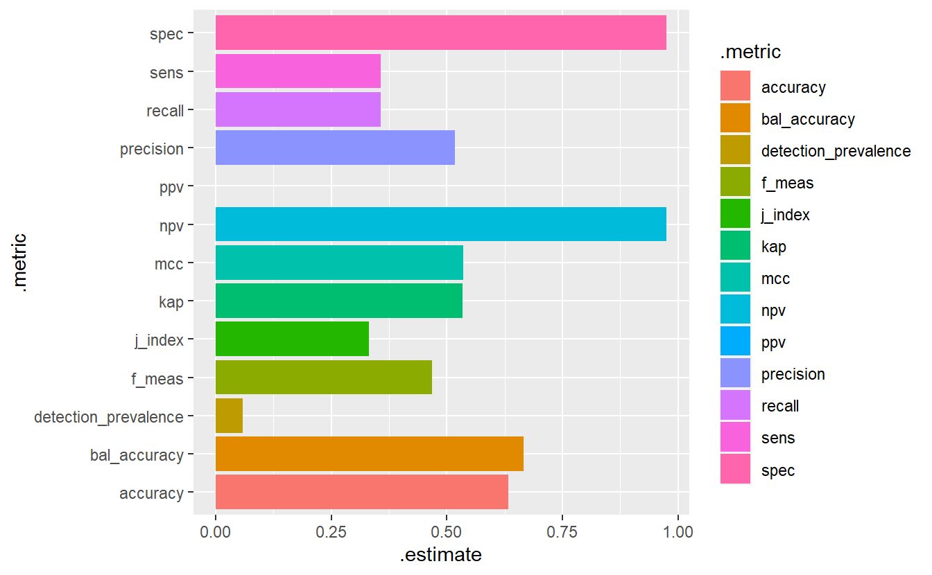

(#fig:5-mm-1 )Model Evaluation Metrics - Base Model

DATA.test.Scored %>%
  mutate(Predict_Correct = if_else(Code_Factor == pred, TRUE, FALSE)) %>%
  ggplot(aes(x=Date_Time, y=Value_Num, color=Predict_Correct)) +
  geom_point()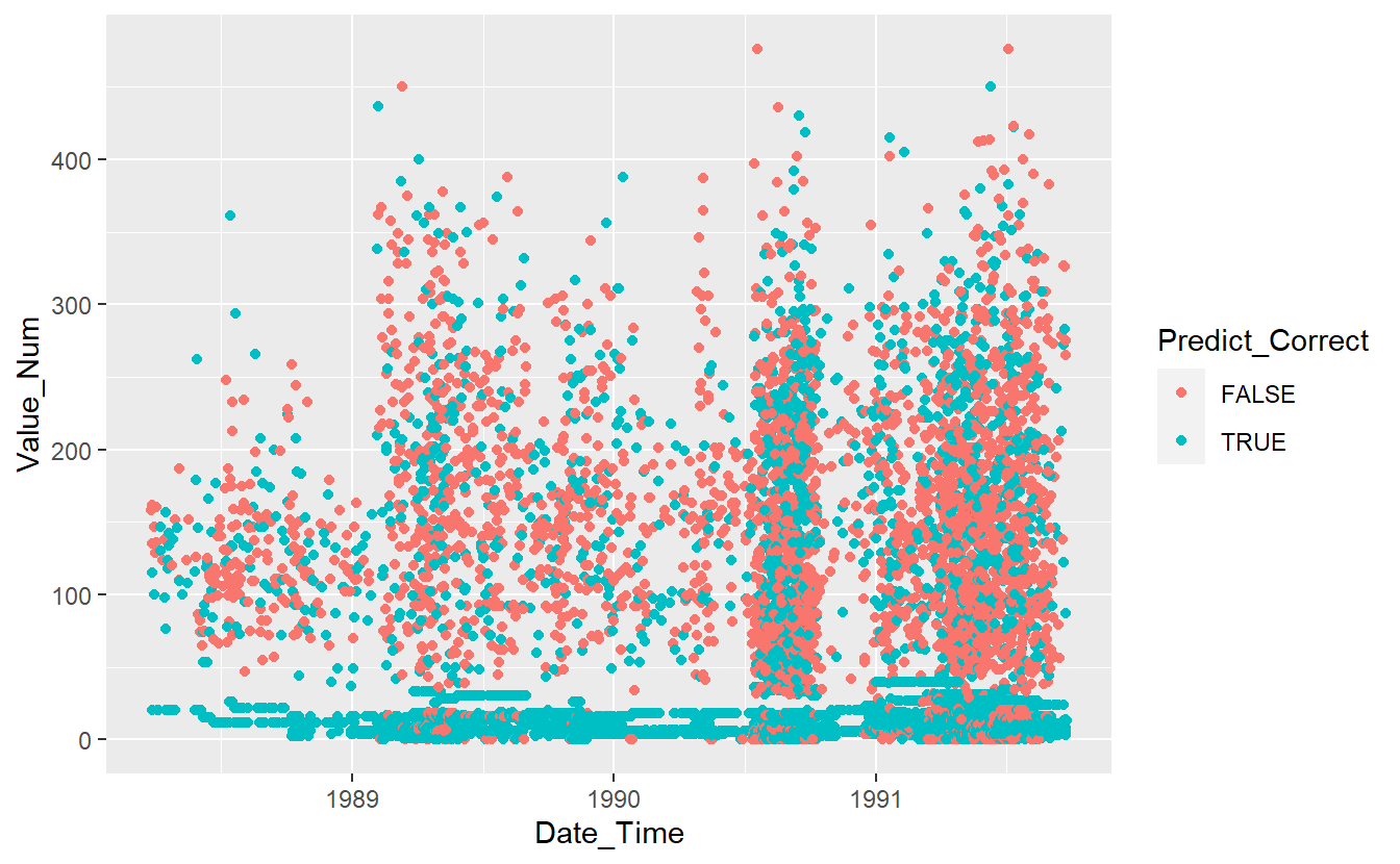

Figure 13.8: Graph of Correct Predictions on test data under base model

\(~\)

13.9 Correlated Probabilites

First, let’s review the probabilities:

Probs <- predict(rf_model, DATA.test.Scored, 'prob') %>%
  as_tibble() 

Probs
#> # A tibble: 10,464 × 17
#>   C_33   C_34  C_35  C_58  C_59  C_60  C_61  C_62  C_63  C_64  C_65  C_66  C_67 
#>   <matr> <mat> <mat> <mat> <mat> <mat> <mat> <mat> <mat> <mat> <mat> <mat> <mat>
#> 1 0.000… 0.00… 0.00… 0.02… 0     0.55… 0     0.37… 0.00… 0.03… 0     0     0    
#> 2 0.250… 0.00… 0.74… 0.00… 0     0.00… 0     0.00… 0.00… 0.00… 0     0     0    
#> 3 0.000… 0.00… 0.00… 0.69… 0     0.16… 0     0.13… 0.00… 0.00… 0     0     0    
#> 4 0.251… 0.01… 0.73… 0.00… 0     0.00… 0     0.00… 0.00… 0.00… 0     0     0    
#> 5 0.000… 0.00… 0.00… 0.31… 0     0.20… 0     0.42… 0.00… 0.05… 0     0     0    
#> 6 0.000… 0.00… 0.00… 0.15… 0     0.28… 0     0.21… 0.28… 0.05… 0     0     0    
#> # … with 10,458 more rows, and 4 more variables: C_68 <matrix>, C_69 <matrix>,
#> #   C_70 <matrix>, C_71 <matrix>

DATA.test.Scored <- cbind(DATA.test.Scored, Probs)

GGally::ggcorr(Probs,
               method = c("pairwise", "pearson"),
               label = TRUE)
#> Registered S3 method overwritten by 'GGally':
#>   method from   
#>   +.gg   ggplot2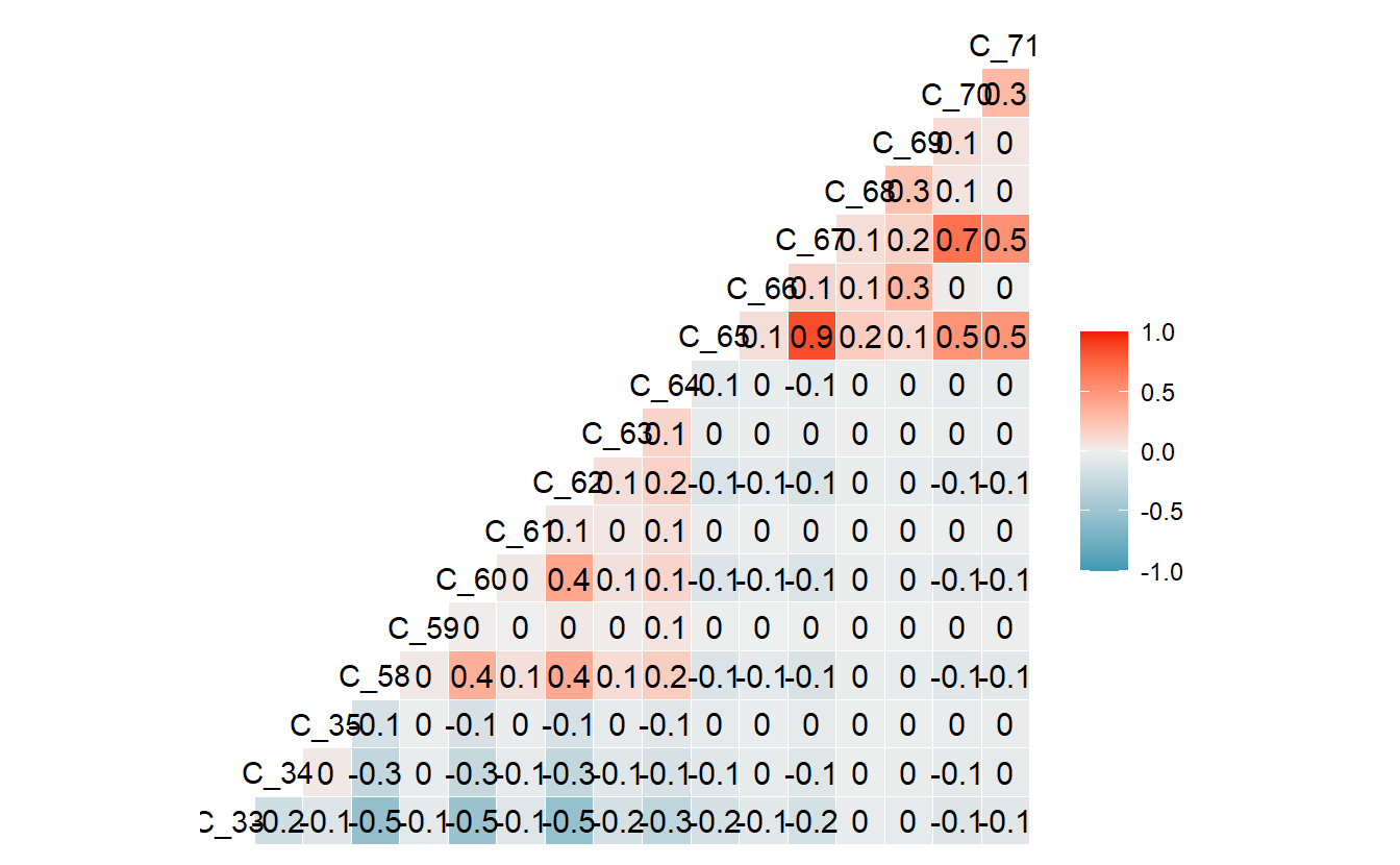

library('corrr')
cor.corr_data <- correlate(Probs)
#> Correlation computed with
#> • Method: 'pearson'
#> • Missing treated using: 'pairwise.complete.obs'

cor.corr_data %>%
  glimpse()
#> Rows: 17
#> Columns: 18
#> $ term <chr> "C_33", "C_34", "C_35", "C_58", "C_59", "C_60", "C_61", "C_62", "…
#> $ C_33 <dbl> NA, -0.19163898, -0.10441614, -0.54956761, -0.05396652, -0.511840…
#> $ C_34 <dbl> -0.19163898, NA, 0.04132957, -0.28371748, -0.02844334, -0.2606538…
#> $ C_35 <dbl> -0.10441614, 0.04132957, NA, -0.14865214, -0.01483954, -0.1393353…
#> $ C_58 <dbl> -0.54956761, -0.28371748, -0.14865214, NA, 0.03561936, 0.36949568…
#> $ C_59 <dbl> -0.053966522, -0.028443345, -0.014839537, 0.035619361, NA, 0.0124…
#> $ C_60 <dbl> -0.51184049, -0.26065388, -0.13933531, 0.36949568, 0.01240024, NA…
#> $ C_61 <dbl> -0.097743416, -0.050999090, -0.023185268, 0.081489225, -0.0013966…
#> $ C_62 <dbl> -0.54217945, -0.27453263, -0.14798142, 0.39238423, 0.03940021, 0.…
#> $ C_63 <dbl> -0.164511288, -0.086079561, -0.045169014, 0.105786617, 0.01077281…
#> $ C_64 <dbl> -0.29676777, -0.14955872, -0.08073562, 0.18846421, 0.05790872, 0.…
#> $ C_65 <dbl> -0.16073437, -0.08587324, -0.04520394, -0.12428883, -0.01218820, …
#> $ C_66 <dbl> -0.066317537, -0.038630694, -0.020294164, -0.056104543, -0.005503…
#> $ C_67 <dbl> -0.16848325, -0.09130119, -0.04765189, -0.13115047, -0.01286117, …
#> $ C_68 <dbl> -0.029782995, -0.015318848, -0.010093123, -0.027725505, -0.002723…
#> $ C_69 <dbl> -0.042576706, -0.026037345, -0.013980500, -0.038633843, -0.003788…
#> $ C_70 <dbl> -0.108371422, -0.059014542, -0.030955034, -0.085714612, -0.008407…
#> $ C_71 <dbl> -0.083580597, -0.048190858, -0.026590249, -0.073846899, -0.007241…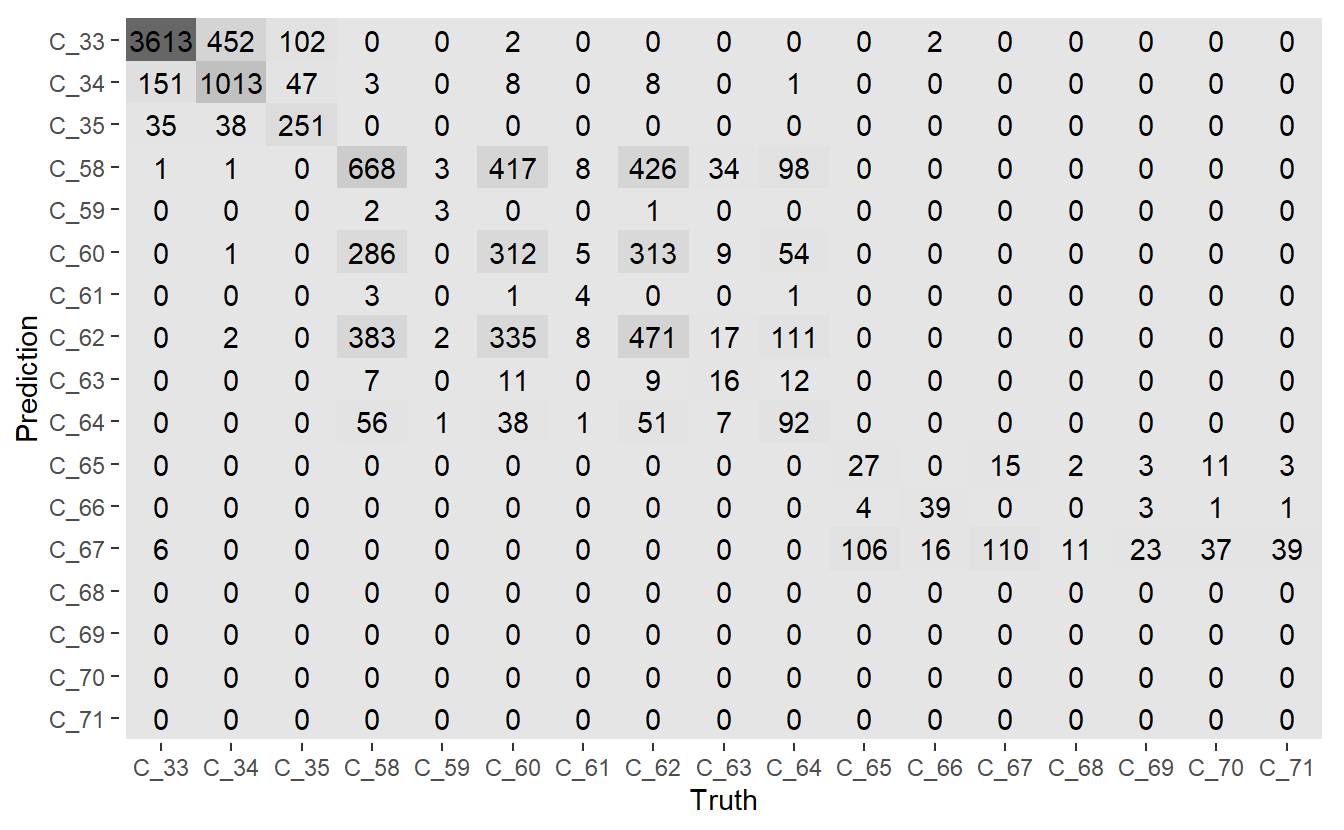

conf_mat.DATA.test.Scored %>%
  autoplot('heatmap')

(#fig:5-corrr-data-heatmap )Heatmap Confusion Matrix of base model

One of the things to note above is that classes C_68, C_69, C_70, C_71 are never predicted.

Likewise the probabilities of C_65, C_70, and C_67 are highly correlated:

cor.corr_data %>%
   filter_at(vars(all_of(colnames(Probs))), any_vars( . > .6 ))
#> # A tibble: 3 × 18
#>   term    C_33    C_34    C_35    C_58     C_59    C_60    C_61    C_62    C_63
#>   <chr>  <dbl>   <dbl>   <dbl>   <dbl>    <dbl>   <dbl>   <dbl>   <dbl>   <dbl>
#> 1 C_65  -0.161 -0.0859 -0.0452 -0.124  -0.0122  -0.116  -0.0221 -0.123  -0.0372
#> 2 C_67  -0.168 -0.0913 -0.0477 -0.131  -0.0129  -0.122  -0.0233 -0.129  -0.0392
#> 3 C_70  -0.108 -0.0590 -0.0310 -0.0857 -0.00841 -0.0798 -0.0152 -0.0846 -0.0256
#> # … with 8 more variables: C_64 <dbl>, C_65 <dbl>, C_66 <dbl>, C_67 <dbl>,
#> #   C_68 <dbl>, C_69 <dbl>, C_70 <dbl>, C_71 <dbl>

And there are a number of classes which do not have many training examples:

DATA.train %>%
  group_by(Code_Factor) %>%
  tally() %>%
  ungroup() %>%
  mutate(n = as.numeric(n)) %>%
  full_join(Code_Table_Factor) %>%
  mutate(n = if_else(is.na(n) , 0 , n)) %>%
  arrange(n) %>%
  print(n=20)
#> Joining, by = "Code_Factor"
#> # A tibble: 17 × 6
#>    Code_Factor     n  Code Code_Description                      Code_…¹ Code_…²
#>    <fct>       <dbl> <dbl> <chr>                                 <lgl>     <dbl>
#>  1 C_59           11    59 Post-breakfast blood glucose measure… FALSE        59
#>  2 C_68           21    68 Less-than-usual meal ingestion        FALSE        68
#>  3 C_69           39    69 Typical exercise activity             FALSE        69
#>  4 C_61           40    61 Post-lunch blood glucose measurement  FALSE        61
#>  5 C_71           55    71 Less-than-usual exercise activity     FALSE        71
#>  6 C_70           90    70 More-than-usual exercise activity     FALSE        70
#>  7 C_66           97    66 Typical meal ingestion                FALSE        66
#>  8 C_63          136    63 Post-supper blood glucose measurement FALSE        63
#>  9 C_65          194    65 Hypoglycemic symptoms                 FALSE        65
#> 10 C_67          201    67 More-than-usual meal ingestion        FALSE        67
#> 11 C_64          535    64 Pre-snack blood glucose measurement   FALSE        64
#> 12 C_35          653    35 UltraLente insulin dose               FALSE        35
#> 13 C_60         1643    60 Pre-lunch blood glucose measurement   FALSE        60
#> 14 C_62         1877    62 Pre-supper blood glucose measurement  FALSE        62
#> 15 C_58         2108    58 Pre-breakfast blood glucose measurem… FALSE        58
#> 16 C_34         2321    34 NPH insulin dose                      FALSE        34
#> 17 C_33         5674    33 Regular insulin dose                  FALSE        33
#> # … with abbreviated variable names ¹Code_Invalid, ²Code_New

Probs.sample <- Probs %>%
  rowwise() %>%
  mutate(rand_num = runif(1)) %>%
  ungroup() %>%
  filter(rand_num > .4) %>%
  select(-rand_num) # this should sample roughly 60% of the Probs data 

nrow(Probs.sample)/nrow(Probs) 
#> [1] 0.5952791

library('broom')
proc.kmeans <- function(data, k = 1:9){

kclusts <-
  tibble(k = k) %>%
  mutate(
    kclust = map(k, ~kmeans(data, .x)),
    glanced = map(kclust, glance),
    augmented = map(kclust, augment, data)
  )

kmeans_model <- function(final_k = 5){
   (kclusts %>%
     filter(k == final_k))$kclust[[1]]
}

id_vars <- colnames(kclusts)

cluster_assignments <- kclusts %>%
  unnest(cols = augmented)

vars <- setdiff(colnames(cluster_assignments), c(id_vars,'.cluster'))

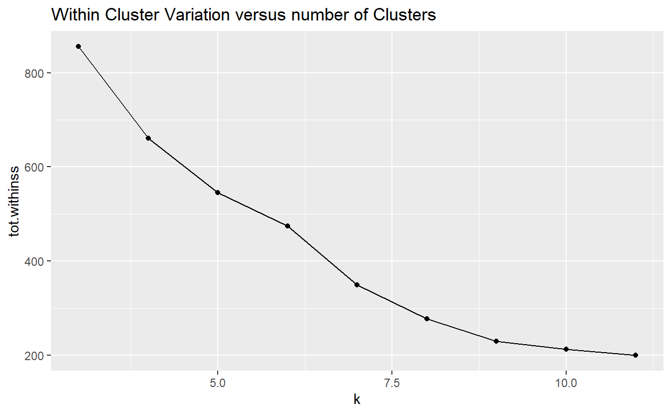
within_cluster_variation_plot <- kclusts %>%
  unnest(cols = c(glanced)) %>%
  ggplot(aes(k, tot.withinss))  +
  geom_line() +
  geom_point() +
  labs(title = "Within Cluster Variation versus number of Clusters")

kmeans.pca <- cluster_assignments %>%
  select(all_of(vars)) %>%
  prcomp()

cluster_assignments_plot <- kmeans.pca %>%
  augment(cluster_assignments) %>%
  ggplot( aes(x = .fittedPC1, y = .fittedPC2, color = .cluster )) +
  geom_point(alpha = 0.8) +
  facet_wrap(~ k) +
  labs(title = "k-means clusterings")

return(list(cluster_assignments_plot= cluster_assignments_plot,
            within_cluster_variation_plot=within_cluster_variation_plot,
            kmeans_model = kmeans_model))
}

proc.kmeans.results <- proc.kmeans(Probs.sample, k=3:11)
proc.kmeans.results
#> $cluster_assignments_plot
#> 
#> $within_cluster_variation_plot
#> 
#> $kmeans_model
#> function(final_k = 5){
#>    (kclusts %>%
#>      filter(k == final_k))$kclust[[1]]
#> }
#> <bytecode: 0x000001ab0dd62f90>
#> <environment: 0x000001ab0d7ee998>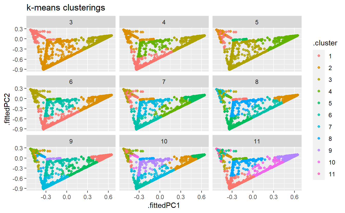

proc.kmeans.results$kmeans_model(6) %>%
  augment(Probs.sample) %>%
  rownames_to_column("id") %>%
  pivot_longer(cols = c(-.cluster, -id), names_to = "class", values_to = "prob") %>%
  mutate(prob = as.numeric(prob)) %>%
  arrange(desc(prob)) %>%
  ggplot(aes(x=class, y=prob, color = .cluster)) +
  geom_point() +
  facet_wrap(~.cluster)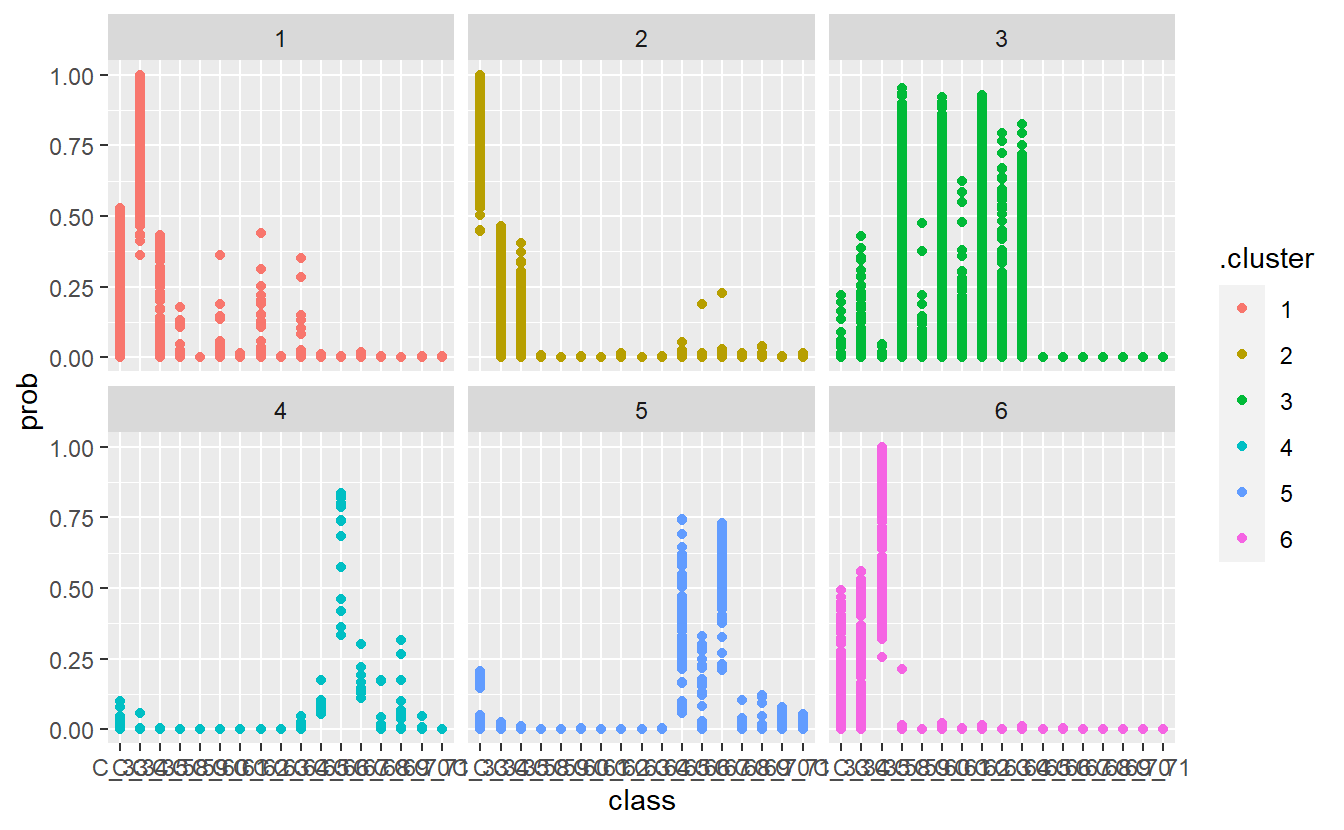

proc.kmeans.results$kmeans_model(6) %>%
  augment(Probs.sample) %>%
  rownames_to_column("id") %>%
  pivot_longer(cols = c(-.cluster, -id), names_to = "class", values_to = "prob") %>%
  mutate(prob = as.numeric(prob)) %>%
  arrange(desc(prob)) %>%
  filter(.cluster == 3) %>%
  ggplot(aes(x=class, y=prob, color = .cluster)) +
  geom_point()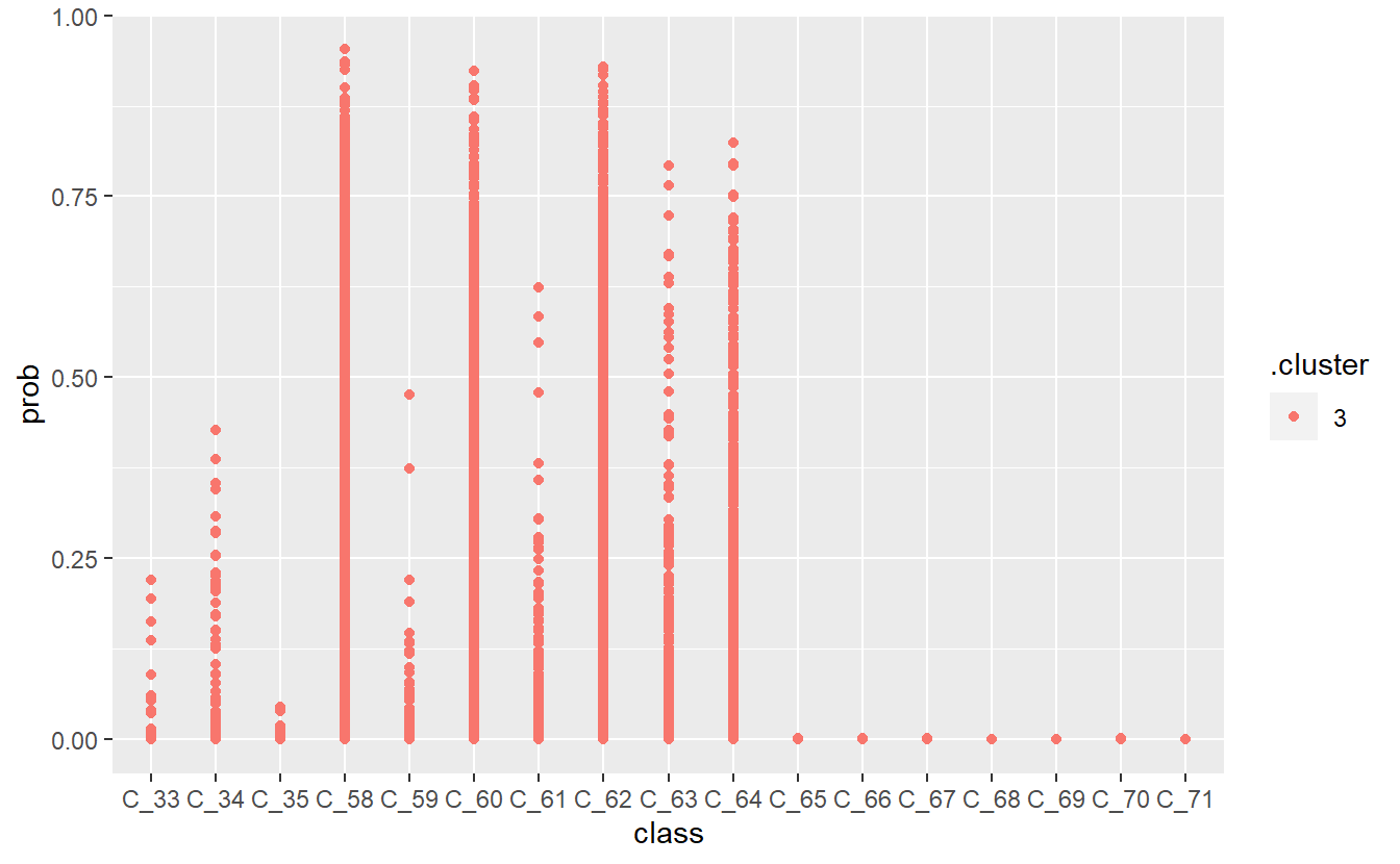

rm(proc.kmeans.results)

saveRDS(rf_model,"DATA/Part_5/models/rf_model.RDS")

rm(rf_model)

13.10 Make Adjustments

Our previous model has some issues, which we can attempt to correct.

Code_Table_Factor_2 <- Code_Table_Factor %>%
  mutate(Code_Description_2 = case_when(
    Code %in% c(33, 34, 35) ~ "insulin dose",
    Code %in% c(58, 60, 62, 64) ~ "pre-meal",
    Code %in% c(59, 61, 63) ~ "post-meal",
    Code %in% c(66, 67, 68, 65) ~ "meal ingestion / Hypoglycemic",
    Code %in% c(69, 70, 71) ~ "exercise activity")
    ) %>%
  mutate(Code_Description_2 = factor(Code_Description_2)) %>%
  select(Code, Code_Description_2)

Code_Table_Factor_2
#> # A tibble: 17 × 2
#>    Code Code_Description_2
#>   <dbl> <fct>             
#> 1    33 insulin dose      
#> 2    34 insulin dose      
#> 3    35 insulin dose      
#> 4    58 pre-meal          
#> 5    59 post-meal         
#> 6    60 pre-meal          
#> # … with 11 more rows

DATA.train_2 <- DATA.train %>% left_join(Code_Table_Factor_2)
#> Joining, by = "Code"

rf_model_2 <- randomForest(Code_Description_2 ~ Date_Time + Value_Num,
                         data = DATA.train_2,
                         ntree = 659,
                         importance = TRUE)

better_rand_forest_errors(rf_model_2)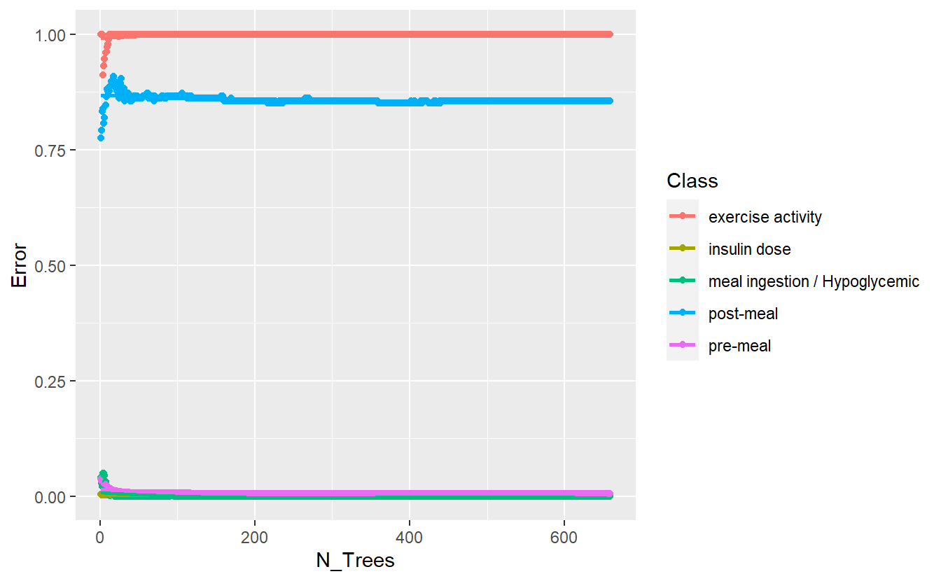

(#fig:5-better-rand-errors-rf-2 )Training Errors on New Model

DATA.test.Scored2 <- DATA.test %>%
  left_join(Code_Table_Factor_2) %>% 
  mutate(model = 'new')
#> Joining, by = "Code"

DATA.test.Scored2$pred <- predict(rf_model_2, DATA.test.Scored2 , 'response')

conf_mat.DATA.test.Scored2 <- DATA.test.Scored2 %>%
  conf_mat(truth = Code_Description_2, pred)

conf_mat.DATA.test.Scored2 %>%
  autoplot('heatmap')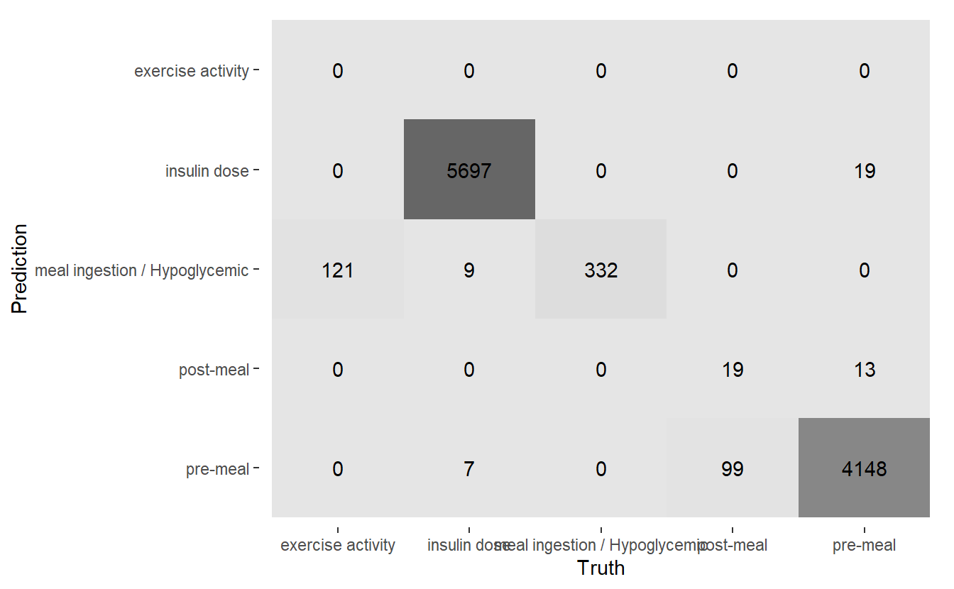

(#fig:5-heatmap-conf-mat-rf-2 )Heatmap Confusion Matrix of New Model

saveRDS(rf_model_2, 'DATA/Part_5/models/rf_model_2.RDS')

base <- DATA.test.Scored %>% conf_mat(truth= Code_Factor, pred) %>% summary() %>% mutate(model = 'base')
#> Warning: While computing multiclass `precision()`, some levels had no predicted events (i.e. `true_positive + false_positive = 0`). 
#> Precision is undefined in this case, and those levels will be removed from the averaged result.
#> Note that the following number of true events actually occured for each problematic event level:
#> 'C_68': 13
#> 'C_69': 29
#> 'C_70': 49
#> 'C_71': 43
#> While computing multiclass `precision()`, some levels had no predicted events (i.e. `true_positive + false_positive = 0`). 
#> Precision is undefined in this case, and those levels will be removed from the averaged result.
#> Note that the following number of true events actually occured for each problematic event level:
#> 'C_68': 13
#> 'C_69': 29
#> 'C_70': 49
#> 'C_71': 43
new <- DATA.test.Scored2 %>% conf_mat(truth= Code_Description_2, pred) %>% summary() %>% mutate(model = 'new')
#> Warning: While computing multiclass `precision()`, some levels had no predicted events (i.e. `true_positive + false_positive = 0`). 
#> Precision is undefined in this case, and those levels will be removed from the averaged result.
#> Note that the following number of true events actually occured for each problematic event level:
#> 'exercise activity': 121
#> Warning: While computing multiclass `precision()`, some levels had no predicted events (i.e. `true_positive + false_positive = 0`). 
#> Precision is undefined in this case, and those levels will be removed from the averaged result.
#> Note that the following number of true events actually occured for each problematic event level:
#> 'exercise activity': 121

comp <- bind_rows(base,
                  new)

comp %>%
  ggplot(aes(x=model, y=.estimate, fill= model)) +
  geom_bar(stat='identity', position = 'dodge') +
  coord_flip() +
  facet_wrap(.metric ~ .)
#> Warning: Removed 2 rows containing missing values (`geom_bar()`).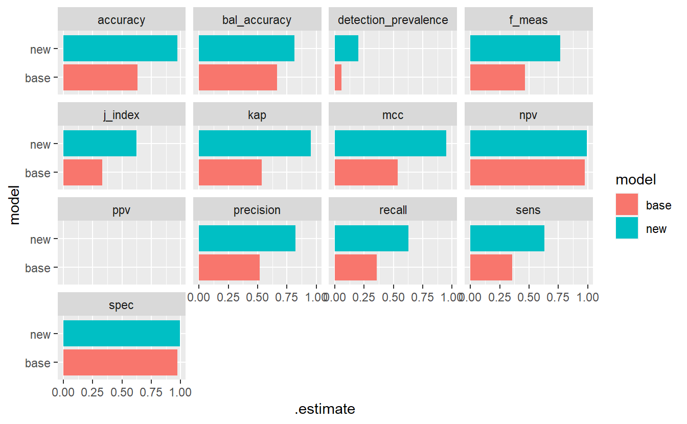

(#fig:5-compare-rf12 )Model Evaluation Metrics - base Vs new model

13.11 Make Adjustments, Again

Let’s make another pass at this, this time we will group together

Code_Table_Factor_3 <- Code_Table_Factor %>%
  mutate(Code_Description_3 = case_when(
    Code %in% c(33, 34, 35) ~ "insulin dose",
    Code %in% c(58, 60, 62, 64, 59, 61, 63) ~ "pre / post meal",
    Code %in% c(66, 67, 68, 65, 69, 70, 71) ~ "meal ingestion / Hypoglycemic / exercise activity")) %>%
  mutate(Code_Description_3 = factor(Code_Description_3)) %>%
  select(Code, Code_Description_3)

Code_Table_Factor_3
#> # A tibble: 17 × 2
#>    Code Code_Description_3
#>   <dbl> <fct>             
#> 1    33 insulin dose      
#> 2    34 insulin dose      
#> 3    35 insulin dose      
#> 4    58 pre / post meal   
#> 5    59 pre / post meal   
#> 6    60 pre / post meal   
#> # … with 11 more rows

DATA.train_3 <- DATA.train %>% left_join(Code_Table_Factor_3)
#> Joining, by = "Code"



rf_model_3 <- randomForest(Code_Description_3 ~ Date_Time + Value_Num,
                         data = DATA.train_3,
                         ntree = 659,
                         importance = TRUE)

rm(DATA.train_3)

better_rand_forest_errors(rf_model_3)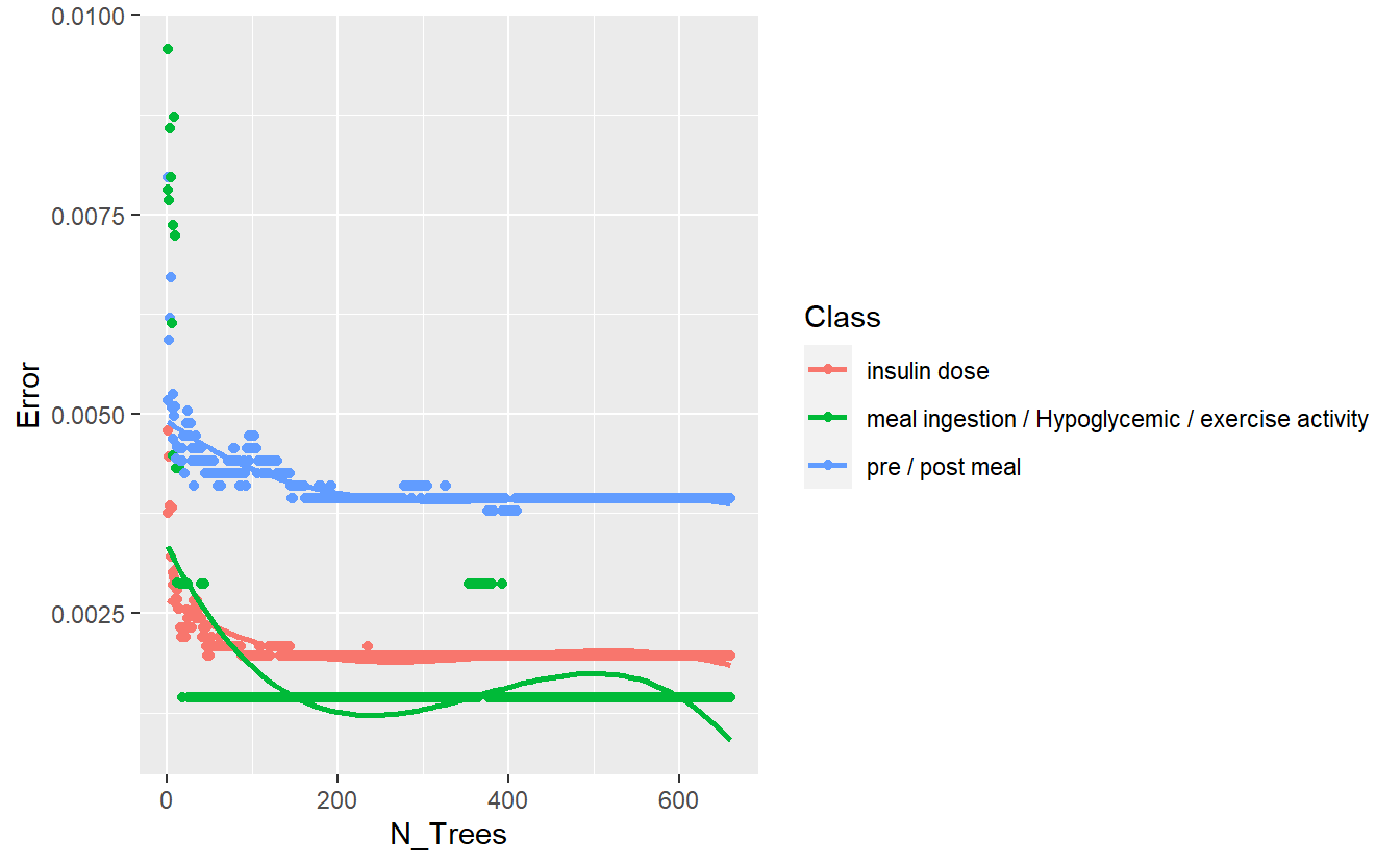

Figure 13.9: Training Errors of Final Model

DATA.test.Scored3 <- DATA.test %>%
  left_join(Code_Table_Factor_3) %>% 
  mutate(model = 'final')
#> Joining, by = "Code"

DATA.test.Scored3$pred <- predict(rf_model_3, DATA.test.Scored3 , 'response')

conf_mat.DATA.test.Scored3 <- DATA.test.Scored3 %>%
  conf_mat(truth = Code_Description_3, pred)

conf_mat.DATA.test.Scored3 %>%
  autoplot('heatmap')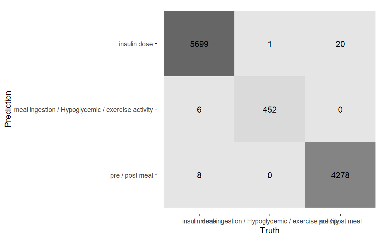

(#fig:5-heatmap-cf-model-rf3 )Heatmap Confusion Matrix of Final Model

saveRDS(rf_model_3, 'DATA/Part_5/models/rf_model_3.RDS')
rm(rf_model_3)

13.12 Extract More Data

library('ggplot2')
library('ggdendro')
library('tree')
#> 
#> Attaching package: 'tree'
#> The following object is masked from 'package:igraph':
#> 
#>     tree

tree_1 <- tree::tree(Code_Factor ~ Date_Time + Value_Num, 
              data = DATA.train)
#> Warning in tree::tree(Code_Factor ~ Date_Time + Value_Num, data = DATA.train):
#> NAs introduced by coercion


plot_dendro_tree <- function(model){

  tree_data <- dendro_data(model)

p <- segment(tree_data) %>%
  ggplot() +
  geom_segment(aes(x = x, 
                   y = y, 
                   xend = xend, 
                   yend = yend, 
                   size = n), 
               colour = "blue", alpha = 0.5) +
  scale_size("n") +
  geom_text(data = label(tree_data), 
            aes(x = x, y = y, label = label), vjust = -0.5, size = 3) +
  geom_text(data = leaf_label(tree_data), 
            aes(x = x, y = y, label = label), vjust = 0.5, size = 2) +
  theme_dendro()
p
}

plot_dendro_tree(tree_1)
#> Warning: Using `size` aesthetic for lines was deprecated in ggplot2 3.4.0.
#> ℹ Please use `linewidth` instead.


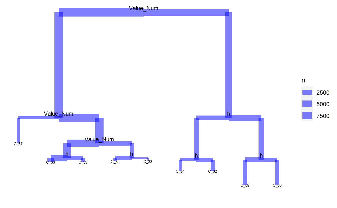
tree_2 <- tree::tree(Code_Factor ~ Date_Time + Value_Num + h + day + month , 
              data = DATA.train_2 %>%
                mutate(h = factor(lubridate::hour(Date_Time))) %>%
                select(Code_Factor, Date_Time, Value_Num, h) %>%
                mutate(day = lubridate::day(Date_Time)) %>%
                mutate(month = month(Date_Time, label = TRUE)) 
)
#> Warning in tree::tree(Code_Factor ~ Date_Time + Value_Num + h + day + month, :
#> NAs introduced by coercion

plot_dendro_tree(tree_2)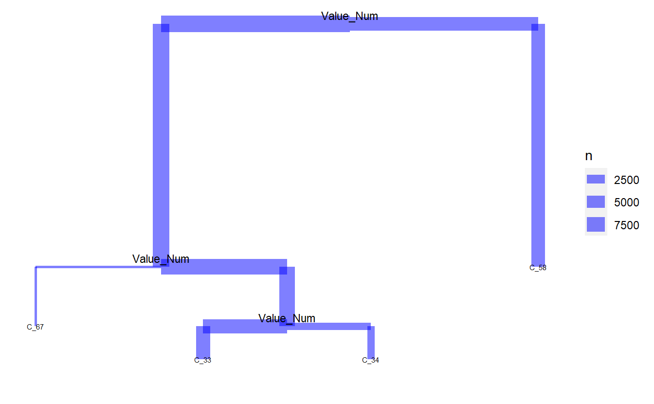

rf_model_4 <- randomForest(Code_Description_2 ~ Date_Time + Value_Num  + h + day + month,
                         data = DATA.train_2 %>%
                mutate(h = factor(lubridate::hour(Date_Time))) %>%
                select(Code_Description_2, Code_Factor, Date_Time, Value_Num, h) %>%
                mutate(day = lubridate::day(Date_Time)) %>%
                mutate(month = month(Date_Time, label = TRUE)),
                         ntree = 659,
                         importance = TRUE)

better_rand_forest_errors(rf_model_4)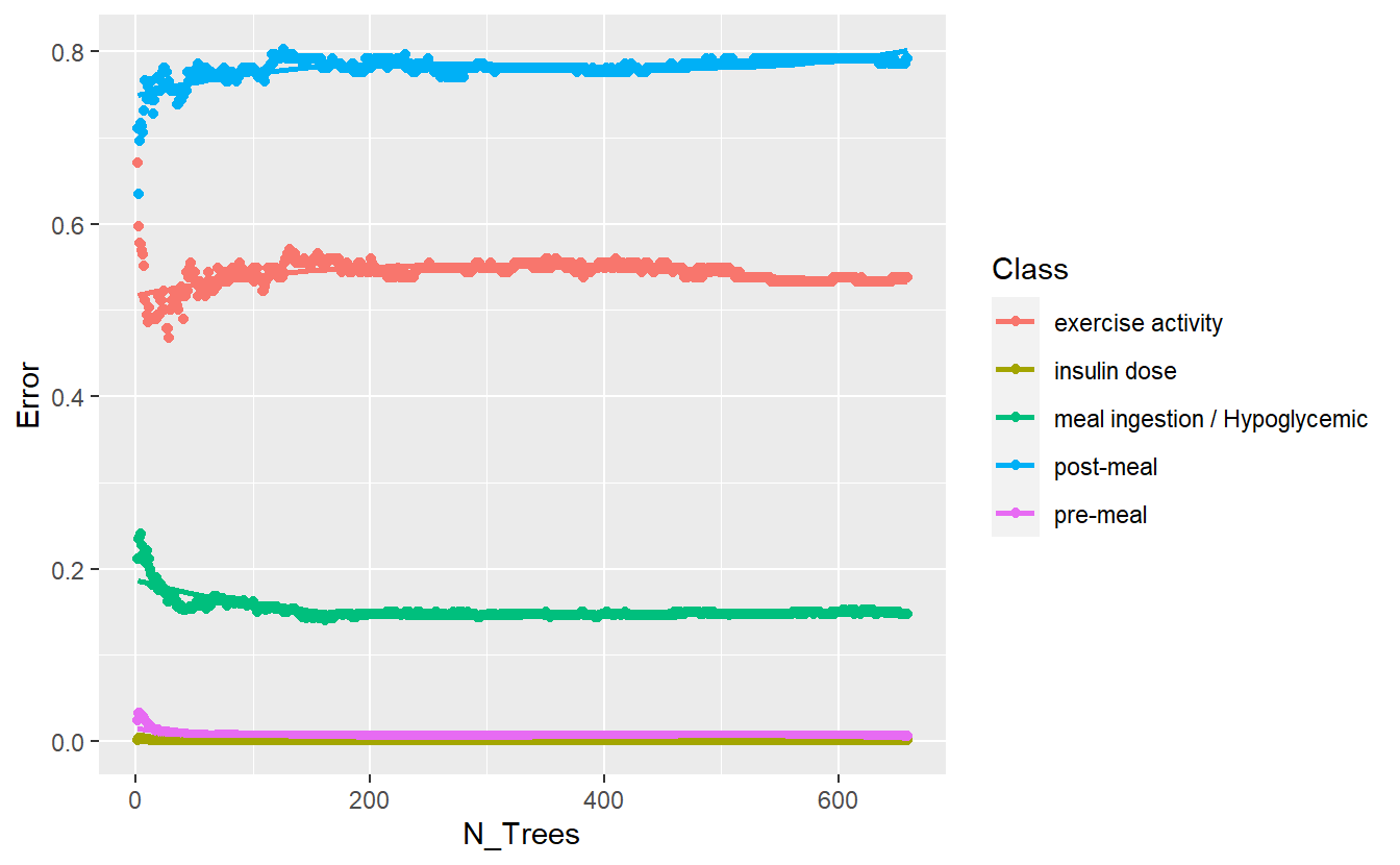

DATA.test.Scored4 <- DATA.test %>%
  left_join(Code_Table_Factor_2) %>% 
  mutate(model = 'final') %>%
  mutate(h = factor(lubridate::hour(Date_Time))) %>%
  mutate(day = lubridate::day(Date_Time)) %>%
  mutate(month = month(Date_Time, label = TRUE)) %>%
  select(Code_Description_2, Code_Factor, Date_Time, Value_Num, day, month, h) 
#> Joining, by = "Code"

DATA.test.Scored4$pred <- predict(rf_model_4, DATA.test.Scored4 , 'response')

conf_mat.DATA.test.Scored4 <- DATA.test.Scored4 %>%
  conf_mat(truth = Code_Description_2, pred)

slim <- conf_mat.DATA.test.Scored3 %>% summary() %>% mutate(model = 'slim')
final <- conf_mat.DATA.test.Scored4 %>% summary() %>% mutate(model = 'final')

comp_f <- bind_rows(comp,
                    slim,
                    final)

comp_f %>%
  ggplot(aes(x=model, y=.estimate, fill = model)) +
  geom_bar(stat='identity', position = 'dodge') + 
  coord_flip() +
  facet_wrap(.metric ~ .)
#> Warning: Removed 2 rows containing missing values (`geom_bar()`).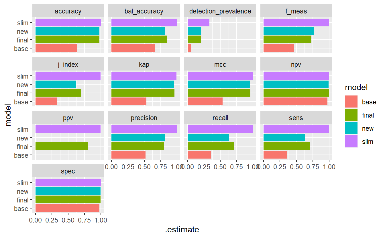

Figure 13.10: Model Evaluation Metrics - base Vs new model Vs Final

13.13 Predict UnKnown Data

keep = c('UnKnown_Measurements','rf_model','rf_model_2','rf_model_3','rf_model_4','keep')

rm(list = setdiff(ls(), keep))

rf_model <- readRDS('DATA/Part_5/models/rf_model.RDS')
rf_model_2 <- readRDS('DATA/Part_5/models/rf_model_2.RDS')
rf_model_3 <- readRDS('DATA/Part_5/models/rf_model_3.RDS')

UnKnown_Measurements$pred_base <- predict(rf_model, UnKnown_Measurements , 'response')
UnKnown_Measurements$pred_new <- predict(rf_model_2, UnKnown_Measurements , 'response')
UnKnown_Measurements$pred_slim <- predict(rf_model_3, UnKnown_Measurements , 'response')

UnKnown_Measurements <- UnKnown_Measurements %>%
  mutate(h = factor(lubridate::hour(Date_Time))) %>%
  mutate(day = lubridate::day(Date_Time)) %>%
  mutate(month = month(Date_Time, label = TRUE))
  

UnKnown_Measurements$pred_final <- predict(rf_model_4, UnKnown_Measurements, 'response')

UnKnown_Measurements %>%
  ggplot(aes(x=Date_Time, y=Value_Num, color=pred_base)) +
  geom_point()
#> Warning: Removed 86 rows containing missing values (`geom_point()`).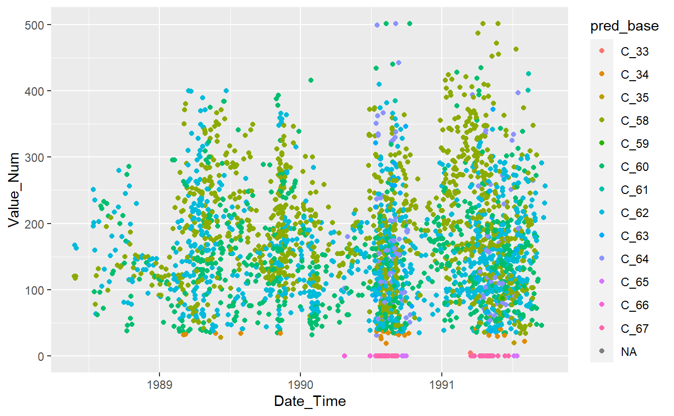

Figure 13.11: Preject UnKnown Data with Base Model

UnKnown_Measurements %>%
  ggplot(aes(x=Date_Time, y=Value_Num, color=pred_new)) +
  geom_point()
#> Warning: Removed 86 rows containing missing values (`geom_point()`).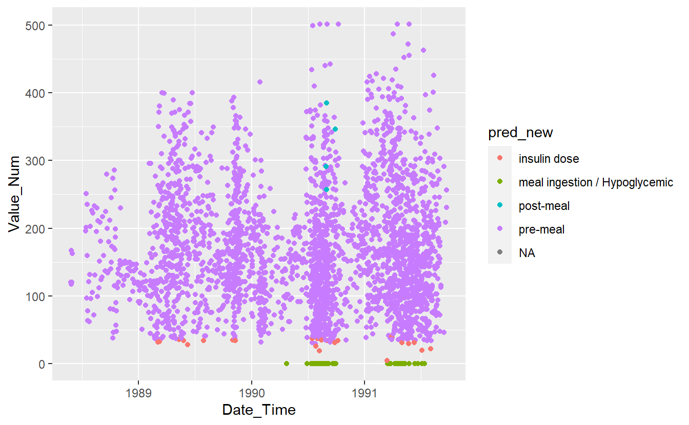

Figure 13.12: Preject UnKnown Data with New Model

UnKnown_Measurements %>%
  ggplot(aes(x=Date_Time, y=Value_Num, color=pred_slim)) +
  geom_point()
#> Warning: Removed 86 rows containing missing values (`geom_point()`).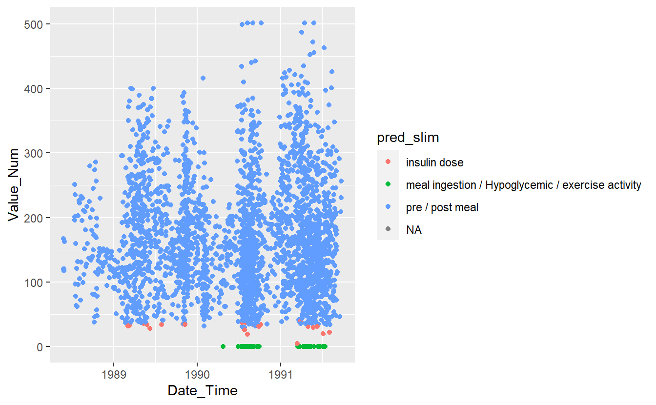

Figure 13.13: Preject UnKnown Data with slim Model

UnKnown_Measurements %>%
  ggplot(aes(x=Date_Time, y=Value_Num, color=pred_final)) +
  geom_point()
#> Warning: Removed 86 rows containing missing values (`geom_point()`).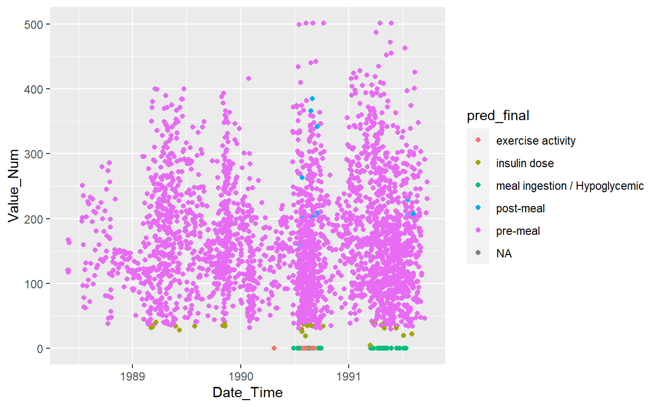

Figure 13.14: Preject UnKnown Data with Final Model

12 Additional Feature Engineering

14 Shiny