1 Getting Started with R

R is a popular programming language within the Data Scientist’s arsenal of tools. R has become popular over the past several years due to its flexibility, various data science uses and it is cost effective. It is widely used due to its array of various uses such as: data wrangling, statistics, machine learning and data visualization. In addition, there is no cost to using R, however there is also no support unless you use a third-party service. Over the course of this text, we will start to get more familiar with R and show how it might be used to complete complicated tasks. Will will be using RStudio as the front-end user interface with R.

1.1 Launch RStudio

Downloading R and RStudio is free. You can download R from https://cran.r-project.org/ and RStudio from https://www.rstudio.com/products/rstudio/ and download the desktop version.

In the first chapter, we introduce you to some base functionality within R and showcase how to perform some basic statistical tasks.

For starters, you can interface directly with the R terminal and enter in basic calculations. Below we show a simple mathematical equation and how R appropriately returns the correct answer:

(2*3-1)^2 - 5 
#> [1] 20

Often we will want to save a value, to do this we use one of the assignment operators: <- , ->, or =, as you can see below the example below:

x <- 2*3
2 -> y 
z = 5
w <- (x-1)^y-z

print(x)
#> [1] 6
print(y)
#> [1] 2
print(z)
#> [1] 5
print(w)
#> [1] 20

1.2 Basic Data Types in R

R has 6 basic data types.

• numeric (real or decimal)
• integer
• character
• logical
• complex

The class function can let you know the data type:

class(3.14)
#> [1] "numeric"
class(pi) # pi = R approximation for pi
#> [1] "numeric"
class(45)
#> [1] "numeric"
class(45L) # add L if you want R to think of this as an integer
#> [1] "integer"
class("integer")
#> [1] "character"
class(TRUE) # logical TRUE
#> [1] "logical"

cx <- complex(length.out = 1, # 1 + 1*sqrt(-1)
        real = 1, 
        imaginary = 1) 

cx
#> [1] 1+1i
class(cx)
#> [1] "complex"

R works with each of these can test if a statement is TRUE or FALSE, for example:

TRUE == FALSE
#> [1] FALSE

1.3 Summary of basic R Data Types

Summary of basic R Data Types

Example	Type
“male,” “Diabetes”	Character / String
3, 20.6, 100.222	Numeric
26L (add an ‘L’ to denote integer)	Integer
TRUE, FALSE	Logical
1+1i	Complex

\(~\)

---

\(~\)

1.4 Lists and Vectors

Lists and vectors are similar in R but a few differences separate them.

List	Vector
A list holds different data such as Numeric, Character, logical, etc.	Vector stores elements of the same type or converts implicitly.
list is a multidimensional object	The vector is one-dimensional
Lists are recursive	vector is not recursive

We can make lists or vectors within R by using the c() function, in the example below we make a few example lists:

list_of_ints <- c(2L,4L,6L,8L)

list_of_strings <- c("Data", "Science", "is a", 'blast!')

list_of_logicals <- c(TRUE, FALSE, TRUE, FALSE)

list_of_mixed_type <- c(3.14, 1L, "cat", TRUE)

list_of_numbers <- c(22/7, 18, 42, 65.2)

list_of_sexes <- c("Male","Female","Female","Male")

R provides many functions to examine features of vectors and other objects, for example

• class() - what kind of object is it (high-level)?
• typeof() - what is the object’s data type (low-level)?
• length() - how long is it? What about two dimensional objects?
• attributes() - does it have any metadata?

class(list_of_strings)
#> [1] "character"
length(list_of_strings)
#> [1] 4
typeof(list_of_strings)
#> [1] "character"
attributes(list_of_strings)
#> NULL

class(list_of_ints)
#> [1] "integer"
length(list_of_ints)
#> [1] 4
typeof(list_of_ints)
#> [1] "integer"
attributes(list_of_ints)
#> NULL

class(list_of_numbers)
#> [1] "numeric"
length(list_of_numbers)
#> [1] 4
typeof(list_of_numbers)
#> [1] "double"
attributes(list_of_numbers)
#> NULL

class(list_of_mixed_type)
#> [1] "character"
length(list_of_mixed_type)
#> [1] 4
typeof(list_of_mixed_type)
#> [1] "character"
attributes(list_of_mixed_type)
#> NULL

1.4.1 Accessing elements in a list

We can access certain elements from within the lists by passing the location of the element of interest within the list:

list_of_mixed_type[1]
#> [1] "3.14"
list_of_mixed_type[2]
#> [1] "1"
list_of_mixed_type[3]
#> [1] "cat"
list_of_mixed_type[4]
#> [1] "TRUE"

list_of_lists <- list(list_of_ints,
                      list_of_strings,
                      list_of_logicals,
                      list_of_mixed_type,
                      list_of_numbers,
                      list_of_sexes)

list_of_lists
#> [[1]]
#> [1] 2 4 6 8
#> 
#> [[2]]
#> [1] "Data"    "Science" "is a"    "blast!" 
#> 
#> [[3]]
#> [1]  TRUE FALSE  TRUE FALSE
#> 
#> [[4]]
#> [1] "3.14" "1"    "cat"  "TRUE"
#> 
#> [[5]]
#> [1]  3.142857 18.000000 42.000000 65.200000
#> 
#> [[6]]
#> [1] "Male"   "Female" "Female" "Male"

list_of_lists[[2]][[4]]
#> [1] "blast!"

names(list_of_lists) <- list('list_of_ints',
                      'list_of_strings',
                      'list_of_logicals',
                      'list_of_mixed_type',
                      'list_of_numbers',
                      'list_of_sexes')

list_of_lists
#> $list_of_ints
#> [1] 2 4 6 8
#> 
#> $list_of_strings
#> [1] "Data"    "Science" "is a"    "blast!" 
#> 
#> $list_of_logicals
#> [1]  TRUE FALSE  TRUE FALSE
#> 
#> $list_of_mixed_type
#> [1] "3.14" "1"    "cat"  "TRUE"
#> 
#> $list_of_numbers
#> [1]  3.142857 18.000000 42.000000 65.200000
#> 
#> $list_of_sexes
#> [1] "Male"   "Female" "Female" "Male"
list_of_lists[['list_of_strings']][[4]]
#> [1] "blast!"

1.4.2 Factors

Factors are the data objects which are used to categorize the data and store it as levels. They can store both strings and integers. They are useful in the columns which have a limited number of unique values. If we use the factor function on list_of_sexes it returns back the list as a factored list with the levels as the unique set of distinct values in the list:

list_of_sexes_factor <- factor(list_of_sexes)
list_of_sexes_factor
#> [1] Male   Female Female Male  
#> Levels: Female Male

1.4.2.1 levels and ordered levels

We can access the levels of a factor with the levels function:

levels(list_of_sexes_factor)
#> [1] "Female" "Male"

The order of the levels in a factor can be changed by applying the factor function again with new order of the levels:

list_of_sexes_factor_relevel <- factor(list_of_sexes, levels = c("Male","Female"))
list_of_sexes_factor_relevel
#> [1] Male   Female Female Male  
#> Levels: Male Female

We can also place an ordering on the factors with the ordered function :

list_of_costs <- c('$0 - $100',
                   '$100 - $200',
                   '$200 - $300',
                   '$300 - $400')

ordered_list_of_costs <- ordered(list_of_costs, levels = list_of_costs)
ordered_list_of_costs
#> [1] $0 - $100   $100 - $200 $200 - $300 $300 - $400
#> Levels: $0 - $100 < $100 - $200 < $200 - $300 < $300 - $400

\(~\)

---

\(~\)

1.5 Matriceis

A matrix (plural matrices) is a rectangular array or table of numbers, symbols, or expressions, arranged in rows and columns, which is used to represent a mathematical object or a property of such an object. In R a matrix \(M\) is an \(n \times k\) array with \(n\) rows with \(k\) columns, we say the dimension of \(M\) is \(n \times k\).

M <- matrix(data = c(1,3,5,2,4,6), nrow = 2, byrow = TRUE)

M
#>      [,1] [,2] [,3]
#> [1,]    1    3    5
#> [2,]    2    4    6

dim(M)
#> [1] 2 3

nrow(M)
#> [1] 2

ncol(M)
#> [1] 3

class(M)
#> [1] "matrix" "array"
length(M)
#> [1] 6
typeof(M)
#> [1] "double"
attributes(M)
#> $dim
#> [1] 2 3

We can also add on additional attributes to the matrix such as dimensional names:

rownames = c("odds", "evens")
colnames = c("col1", "col2", "col3")

M <- matrix(data = c(1,3,5,2,4,6), nrow = 2, byrow = TRUE, dimnames = list(rownames, colnames))
M
#>       col1 col2 col3
#> odds     1    3    5
#> evens    2    4    6

class(M)
#> [1] "matrix" "array"
length(M)
#> [1] 6
typeof(M)
#> [1] "double"
attributes(M)
#> $dim
#> [1] 2 3
#> 
#> $dimnames
#> $dimnames[[1]]
#> [1] "odds"  "evens"
#> 
#> $dimnames[[2]]
#> [1] "col1" "col2" "col3"

\(~\)

---

\(~\)

1.6 The Data Frame

A Data Frame is a two-dimensional array-like structure in which each column contains values of one variable and each row contains one set of values from each column.

my_dataframe <- data.frame(list_of_ints, 
                           list_of_strings, 
                           list_of_logicals, 
                           list_of_mixed_type, 
                           list_of_numbers,
                           list_of_sexes_factor,
                           ordered_list_of_costs)

my_dataframe
#>   list_of_ints list_of_strings list_of_logicals list_of_mixed_type
#> 1            2            Data             TRUE               3.14
#> 2            4         Science            FALSE                  1
#> 3            6            is a             TRUE                cat
#> 4            8          blast!            FALSE               TRUE
#>   list_of_numbers list_of_sexes_factor ordered_list_of_costs
#> 1        3.142857                 Male             $0 - $100
#> 2       18.000000               Female           $100 - $200
#> 3       42.000000               Female           $200 - $300
#> 4       65.200000                 Male           $300 - $400

class(my_dataframe)
#> [1] "data.frame"
length(my_dataframe)
#> [1] 7
typeof(my_dataframe)
#> [1] "list"
attributes(my_dataframe)
#> $names
#> [1] "list_of_ints"          "list_of_strings"       "list_of_logicals"     
#> [4] "list_of_mixed_type"    "list_of_numbers"       "list_of_sexes_factor" 
#> [7] "ordered_list_of_costs"
#> 
#> $class
#> [1] "data.frame"
#> 
#> $row.names
#> [1] 1 2 3 4

The primary difference between dataframes and matrices is that dataframes allow for columns to be of different datatypes.

We can see the first few rows of a dataframe with the head function:

head(my_dataframe)
#>   list_of_ints list_of_strings list_of_logicals list_of_mixed_type
#> 1            2            Data             TRUE               3.14
#> 2            4         Science            FALSE                  1
#> 3            6            is a             TRUE                cat
#> 4            8          blast!            FALSE               TRUE
#>   list_of_numbers list_of_sexes_factor ordered_list_of_costs
#> 1        3.142857                 Male             $0 - $100
#> 2       18.000000               Female           $100 - $200
#> 3       42.000000               Female           $200 - $300
#> 4       65.200000                 Male           $300 - $400

1.6.0.1 The dim function

We can determine the dimension by using the dim function:

dim(my_dataframe)
#> [1] 4 7

so we can see that this data-frame has 4 rows and 7 columns. We can also get those values by using nrow and ncol:

nrow(my_dataframe)
#> [1] 4

ncol(my_dataframe)
#> [1] 7

1.6.1 Matrix Notation

We can use familiar matrix notation to select specific elements from the data frame:

my_dataframe[3,5]
#> [1] 42

We can use similar notation to select a row:

my_dataframe[3,]
#>   list_of_ints list_of_strings list_of_logicals list_of_mixed_type
#> 3            6            is a             TRUE                cat
#>   list_of_numbers list_of_sexes_factor ordered_list_of_costs
#> 3              42               Female           $200 - $300

Or a column:

my_dataframe[,5]
#> [1]  3.142857 18.000000 42.000000 65.200000

1.6.2 Data Frames have colnames

It is important to have meaningful column names in our dataframe. This is useful for quickly understanding what variables you are viewing and logical for programming purposes. You can review the column names of a dataframe with the colnames functions:

colnames(my_dataframe)
#> [1] "list_of_ints"          "list_of_strings"       "list_of_logicals"     
#> [4] "list_of_mixed_type"    "list_of_numbers"       "list_of_sexes_factor" 
#> [7] "ordered_list_of_costs"

It is also helpful to be able to pass in these column names to select a column rather than recall which column number the information is associated with:

my_dataframe[,'list_of_ints']
#> [1] 2 4 6 8

We may also use the following code to access a column in a dataframe:

my_dataframe$list_of_strings
#> [1] "Data"    "Science" "is a"    "blast!"

\(~\)

---

\(~\)

1.7 Structure

The R Structure function will compactly display the internal structure of an R object.

To see help page for a function use ? before the function name, for example try: ?str

For example, if we use str on my_dataframe it will show the user the number of observations, variables and data type of each list:

str(my_dataframe)
#> 'data.frame':    4 obs. of  7 variables:
#>  $ list_of_ints         : int  2 4 6 8
#>  $ list_of_strings      : chr  "Data" "Science" "is a" "blast!"
#>  $ list_of_logicals     : logi  TRUE FALSE TRUE FALSE
#>  $ list_of_mixed_type   : chr  "3.14" "1" "cat" "TRUE"
#>  $ list_of_numbers      : num  3.14 18 42 65.2
#>  $ list_of_sexes_factor : Factor w/ 2 levels "Female","Male": 2 1 1 2
#>  $ ordered_list_of_costs: Ord.factor w/ 4 levels "$0 - $100"<"$100 - $200"<..: 1 2 3 4

When we call str on list_of_costs we see that it is a character vector of length 4 and are shown the values

str(list_of_costs)
#>  chr [1:4] "$0 - $100" "$100 - $200" "$200 - $300" "$300 - $400"

\(~\)

---

\(~\)

1.8 summary

The summary is a generic function used to produce summaries of the results of various model fitting functions.

See ?summary for more information.

In the case of a dataframe the summary function will give summary level information on the dataframe, for continuous variables it will display the minimum, first quartile, median, mean, third quartile and max; for categorical data counts of each of the classes

summary(my_dataframe)
#>   list_of_ints list_of_strings    list_of_logicals list_of_mixed_type
#>  Min.   :2.0   Length:4           Mode :logical    Length:4          
#>  1st Qu.:3.5   Class :character   FALSE:2          Class :character  
#>  Median :5.0   Mode  :character   TRUE :2          Mode  :character  
#>  Mean   :5.0                                                         
#>  3rd Qu.:6.5                                                         
#>  Max.   :8.0                                                         
#>  list_of_numbers  list_of_sexes_factor ordered_list_of_costs
#>  Min.   : 3.143   Female:2             $0 - $100  :1        
#>  1st Qu.:14.286   Male  :2             $100 - $200:1        
#>  Median :30.000                        $200 - $300:1        
#>  Mean   :32.086                        $300 - $400:1        
#>  3rd Qu.:47.800                                             
#>  Max.   :65.200

We can also get these statistics by class, here we use the information in the dataframe column list_of_sexes

by(my_dataframe, my_dataframe$list_of_sexes, summary)
#> my_dataframe$list_of_sexes: Female
#>   list_of_ints list_of_strings    list_of_logicals list_of_mixed_type
#>  Min.   :4.0   Length:2           Mode :logical    Length:2          
#>  1st Qu.:4.5   Class :character   FALSE:1          Class :character  
#>  Median :5.0   Mode  :character   TRUE :1          Mode  :character  
#>  Mean   :5.0                                                         
#>  3rd Qu.:5.5                                                         
#>  Max.   :6.0                                                         
#>  list_of_numbers list_of_sexes_factor ordered_list_of_costs
#>  Min.   :18      Female:2             $0 - $100  :0        
#>  1st Qu.:24      Male  :0             $100 - $200:1        
#>  Median :30                           $200 - $300:1        
#>  Mean   :30                           $300 - $400:0        
#>  3rd Qu.:36                                                
#>  Max.   :42                                                
#> ------------------------------------------------------------ 
#> my_dataframe$list_of_sexes: Male
#>   list_of_ints list_of_strings    list_of_logicals list_of_mixed_type
#>  Min.   :2.0   Length:2           Mode :logical    Length:2          
#>  1st Qu.:3.5   Class :character   FALSE:1          Class :character  
#>  Median :5.0   Mode  :character   TRUE :1          Mode  :character  
#>  Mean   :5.0                                                         
#>  3rd Qu.:6.5                                                         
#>  Max.   :8.0                                                         
#>  list_of_numbers  list_of_sexes_factor ordered_list_of_costs
#>  Min.   : 3.143   Female:0             $0 - $100  :1        
#>  1st Qu.:18.657   Male  :2             $100 - $200:0        
#>  Median :34.171                        $200 - $300:0        
#>  Mean   :34.171                        $300 - $400:1        
#>  3rd Qu.:49.686                                             
#>  Max.   :65.200

\(~\)

---

\(~\)

1.9 Save and Read RDS files

You can save important data, variables, or models as R data files using saveRDS:

saveRDS(my_dataframe,'my_dataframe.RDS')

by default this saves to your working directory.

1.10 getwd()

You can see your current working directory path by using getwd():

getwd()
#> [1] "C:/Users/jkyle/Documents/GitHub/Jeff_Data_Wrangling"

You can alter the paths in a number of different ways.

In this example, we will want to save results to a sub-folder called y_data.

First, I will tell R to create a directory:

new_path <- file.path(getwd(),'y_data')

dir.create(new_path)

Now I can save y within this folder:

saveRDS(y, file.path(new_path,'y.RDS'))

1.11 readRDS

You can load R data files by using readRDS:

z <- readRDS(file.path(new_path, 'y.RDS'))

y == z
#> [1] TRUE

\(~\)

---

\(~\)

1.12 Remove Items from your enviroment

WARNING once something is removed from your environment it is GONE! SAVE WHAT YOU NEED with saveRDS otherwise you will need to rerun portions of code.

You can remove items in your R environment by using the rm function.

rm(my_dataframe2)
#> Warning in rm(my_dataframe2): object 'my_dataframe2' not found

1.12.1 Remove all but a list

Let’s say that we want to remove everything except for my_dataframe and y, then we might do something like:

keep <- c('my_dataframe','new_path')

rm(list = setdiff(ls(), keep))

Above we are using multiple functions in conjunction with one-another:

1. We make a variable called keep to contain the items we wish to maintain
2. ls is returning a list of items within the environment
3. setdiff is taking the set-difference between ls which returns all the items within the environment and the items that we have specified within keep.

1.12.2 Delete Files / Folders

unlink deletes a file, we can use recursive = TRUE to delete directories:

unlink(new_path, recursive = TRUE)

\(~\)

---

\(~\)

1.13 Functions

A function is an R object that takes in arguments or parameters and follows the collection of statements to provide the requested return.

1.13.1 Example R functions.

The R function set.seed is designed to assist with pseudo-random number generation.

The R function rnorm will produce a given number of randomly generated numbers with a provided mean and standard-deviation, Below we define 3 distributions each of 1000 numbers:

• X, Y, and Z will be drawn from a distribution with mean of 0 and standard deviation of 1.
• X and Z will be drawn with the same seed where as Y will be drawn with a different seed.
• Y will be drawn from a distribution with mean of 5 and standard deviation of 2.

{
set.seed(12345)
X <- rnorm(1000, mean = 0, sd = 1)
}

{
set.seed(5)
Y <- rnorm(1000, mean = 0, sd = 1)
W <- rnorm(1000, mean = 5, sd = 2)
}


{
set.seed(12345)
Z <- rnorm(1000, mean = 0, sd = 1)
}

Here are the first 10 from each of the distributions:

cat("X \n")
#> X
X[1:10]
#>  [1]  0.5855288  0.7094660 -0.1093033 -0.4534972  0.6058875 -1.8179560
#>  [7]  0.6300986 -0.2761841 -0.2841597 -0.9193220

cat("Y \n")
#> Y
Y[1:10]
#>  [1] -0.84085548  1.38435934 -1.25549186  0.07014277  1.71144087 -0.60290798
#>  [7] -0.47216639 -0.63537131 -0.28577363  0.13810822

cat("W \n")
#> W
W[1:10]
#>  [1] 2.089891 7.489126 4.136106 5.013739 5.249102 4.180743 6.126827 8.213916
#>  [9] 2.996097 6.018652

cat("Z \n")
#> Z
Z[1:10]
#>  [1]  0.5855288  0.7094660 -0.1093033 -0.4534972  0.6058875 -1.8179560
#>  [7]  0.6300986 -0.2761841 -0.2841597 -0.9193220

Note that X and Z will be exactly the same sets since we used the same seed to generate the two sets of numbers whereas Y will be different, even though we used the same parameters, for example

X[546] == Z[546]
#> [1] TRUE
X[546] == Y[546]
#> [1] FALSE

Even though X and Y are not the same, they are sampled from the same distribution therefore the p-value on the t-test should be well above .05:

t.test(X,Y)
#> 
#>  Welch Two Sample t-test
#> 
#> data:  X and Y
#> t = 0.6405, df = 1997.7, p-value = 0.5219
#> alternative hypothesis: true difference in means is not equal to 0
#> 95 percent confidence interval:
#>  -0.05938059  0.11697799
#> sample estimates:
#>  mean of x  mean of y 
#> 0.04619816 0.01739946

Comparatively, X and W were not sampled from the same distribution, therefore the p-value should be closer to 0:

t.test(X,W)
#> 
#>  Welch Two Sample t-test
#> 
#> data:  X and W
#> t = -72.569, df = 1474.2, p-value < 2.2e-16
#> alternative hypothesis: true difference in means is not equal to 0
#> 95 percent confidence interval:
#>  -5.237795 -4.962086
#> sample estimates:
#>  mean of x  mean of y 
#> 0.04619816 5.14613865

We can see the difference between the distributions by using the hist function:

hist(X, col=rgb(1,0,0,0.5), main="Overlapping Histogram") # red
hist(Y, col=rgb(0,1,0,0.5) , add=T) # green
hist(W, col=rgb(0,0,1,0.5) , add=T) # blue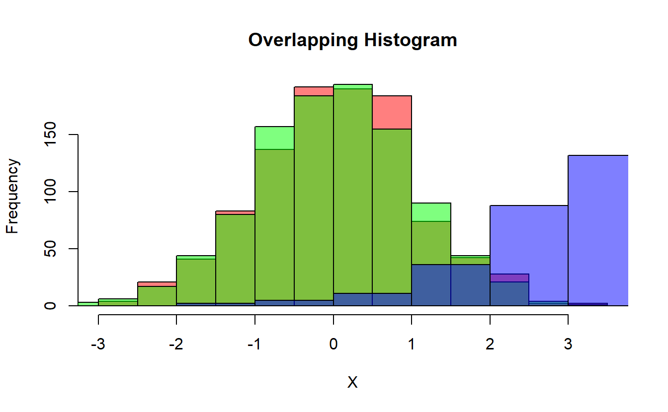 

(#fig:hist1 )Overlapping Histogram of X, Y, & W

1.14 User defined functions

Many of you may recall the quadratic formula from algebra; given a general quadratic equation of the form:

\[ax^2 + bx + c = 0 \]

with \(a\), \(b\), and \(c\) representing constants with \(a \neq 0\) then

\[x = -b \pm \frac{\sqrt{b^2 - 4ac}}{2a}\]

are the two solutions or roots of the quadratic equation.

We can program an R function that takes in as inputs the coefficients from a quadratic equation and returns the two solutions:

quadratic_forumla <- function(a,b,c){
  x_1 <- (-b + sqrt(b^2 - 4*a*c))/(2*a)
  x_2 <- (-b - sqrt(b^2 - 4*a*c))/(2*a)
return(c(x_2,x_1))
}

quadratic_forumla(1,5,6)
#> [1] -3 -2

quadratic_forumla(5,3,-10)
#> [1] -1.745683  1.145683

quadratic_forumla(2,5,3)
#> [1] -1.5 -1.0

\(~\)

---

\(~\)

1.15 Libraries & Packages

You may want to use newer or more specialized packages or libraries to read in or handle data. First you will need to make sure the library is installed with install.packages('package_name') then you can load the library with library('package_name') , and you will have access to all of the functionality withing the package.

Additionally, we can access a function from a library without loading the entire library, this can be done by using a command such as package::function, for instance, readr::read_csv tells R to look in the readr package for the function read_csv. This can be useful in programming functions and packages as well as if multiple packages contain functions with the same name.

1.15.1 installed packages

To see which packages are installed on your machine you can use:

# which packages are installed
library()$results[,1]

sample(library()$results[,1], 20, replace = FALSE)
#>  [1] "bitops"      "clock"       "htmlwidgets" "crayon"      "inum"       
#>  [6] "recipes"     "askpass"     "viridisLite" "ranger"      "tools"      
#> [11] "remotes"     "modelr"      "gtools"      "skimr"       "labeling"   
#> [16] "grid"        "backports"   "dbplyr"      "rstudioapi"  "mgcv"

The following function will check if a list of packages are already installed, if not then it will install them:

# install package if missing 
install_if_not <- function( list.of.packages ) {

  new.packages <- list.of.packages[!(list.of.packages %in% installed.packages()[,"Package"])]
  
  if(length(new.packages)) { install.packages(new.packages, repos = "http://cran.us.r-project.org") } else { print(paste0("the package '", list.of.packages , "' is already installed")) }
}

You can use the function like this:

# test function
install_if_not(c("tidyverse"))
#> [1] "the package 'tidyverse' is already installed"

some additional information on the installed packages including the version can be found now:

tibble::as_tibble(installed.packages())
#> # A tibble: 292 × 16
#>   Package    LibPath     Version Prior…¹ Depends Imports Linki…² Sugge…³ Enhan…⁴
#>   <chr>      <chr>       <chr>   <chr>   <chr>   <chr>   <chr>   <chr>   <chr>  
#> 1 abind      C:/Users/j… 1.4-5   <NA>    R (>= … method… <NA>     <NA>   <NA>   
#> 2 Amelia     C:/Users/j… 1.8.1   <NA>    R (>= … foreig… Rcpp (… "tcltk… <NA>   
#> 3 AMR        C:/Users/j… 1.8.2   <NA>    R (>= … <NA>    <NA>    "curl,… cleane…
#> 4 arsenal    C:/Users/j… 3.6.3   <NA>    R (>= … knitr … <NA>    "broom… <NA>   
#> 5 askpass    C:/Users/j… 1.1     <NA>    <NA>    sys (>… <NA>    "testt… <NA>   
#> 6 assertthat C:/Users/j… 0.2.1   <NA>    <NA>    tools   <NA>    "testt… <NA>   
#> # … with 286 more rows, 7 more variables: License <chr>, License_is_FOSS <chr>,
#> #   License_restricts_use <chr>, OS_type <chr>, MD5sum <chr>,
#> #   NeedsCompilation <chr>, Built <chr>, and abbreviated variable names
#> #   ¹​Priority, ²​LinkingTo, ³​Suggests, ⁴​Enhances

1.15.2 loaded packages

To check which packages are loaded you can use:

# loaded packages
(.packages())
#> [1] "stats"     "graphics"  "grDevices" "utils"     "datasets"  "methods"  
#> [7] "base"

Make sure that the tidyverse and dplyr packages are installed. You can run install.packages(c('tidyverse','dplyr')) to install both.

1.15.3 read sample data

my_dataframe <- readRDS('my_dataframe.RDS' )

We can use the head command to see the first few rows:

head(my_dataframe)
#>   list_of_ints list_of_strings list_of_logicals list_of_mixed_type
#> 1            2            Data             TRUE               3.14
#> 2            4         Science            FALSE                  1
#> 3            6            is a             TRUE                cat
#> 4            8          blast!            FALSE               TRUE
#>   list_of_numbers list_of_sexes_factor ordered_list_of_costs
#> 1        3.142857                 Male             $0 - $100
#> 2       18.000000               Female           $100 - $200
#> 3       42.000000               Female           $200 - $300
#> 4       65.200000                 Male           $300 - $400

\(~\)

---

\(~\)

1.16 Using Packages

We make sections of code accessible to installed packages by using library command:

loaded_package_before <- (.packages())

# everthing below here can call functions in dplyr package
library('dplyr')
#> 
#> Attaching package: 'dplyr'
#> The following objects are masked from 'package:stats':
#> 
#>     filter, lag
#> The following objects are masked from 'package:base':
#> 
#>     intersect, setdiff, setequal, union

glimpse(my_dataframe)
#> Rows: 4
#> Columns: 7
#> $ list_of_ints          <int> 2, 4, 6, 8
#> $ list_of_strings       <chr> "Data", "Science", "is a", "blast!"
#> $ list_of_logicals      <lgl> TRUE, FALSE, TRUE, FALSE
#> $ list_of_mixed_type    <chr> "3.14", "1", "cat", "TRUE"
#> $ list_of_numbers       <dbl> 3.142857, 18.000000, 42.000000, 65.200000
#> $ list_of_sexes_factor  <fct> Male, Female, Female, Male
#> $ ordered_list_of_costs <ord> $0 - $100, $100 - $200, $200 - $300, $300 - $400

(.packages())
#> [1] "dplyr"     "stats"     "graphics"  "grDevices" "utils"     "datasets" 
#> [7] "methods"   "base"

loaded_package_after <- (.packages())

setdiff(loaded_package_after, loaded_package_before)
#> [1] "dplyr"

detach(package:dplyr)
#the dplyr package has now been detached. calls to functions may have errors

packages_cur <- (.packages())

setdiff(loaded_package_after,packages_cur)
#> [1] "dplyr"

Additionally, we can access a function from a library without loading the entire library, this can be done by using a command such as package::function. This notation is needed in any instance where two or more loaded packages have at least one function with the same name. This notation is also useful in development of functions and packages.

For instance, the glimpse function from the dplyr package can also be accessed by using the following command

# glimpse the data
dplyr::glimpse(my_dataframe)
#> Rows: 4
#> Columns: 7
#> $ list_of_ints          <int> 2, 4, 6, 8
#> $ list_of_strings       <chr> "Data", "Science", "is a", "blast!"
#> $ list_of_logicals      <lgl> TRUE, FALSE, TRUE, FALSE
#> $ list_of_mixed_type    <chr> "3.14", "1", "cat", "TRUE"
#> $ list_of_numbers       <dbl> 3.142857, 18.000000, 42.000000, 65.200000
#> $ list_of_sexes_factor  <fct> Male, Female, Female, Male
#> $ ordered_list_of_costs <ord> $0 - $100, $100 - $200, $200 - $300, $300 - $400

And just notice that without the library loaded or the dplyr:: in front we can error:

# error
glimpse(my_dataframe)
#> Rows: 4
#> Columns: 7
#> $ list_of_ints          <int> 2, 4, 6, 8
#> $ list_of_strings       <chr> "Data", "Science", "is a", "blast!"
#> $ list_of_logicals      <lgl> TRUE, FALSE, TRUE, FALSE
#> $ list_of_mixed_type    <chr> "3.14", "1", "cat", "TRUE"
#> $ list_of_numbers       <dbl> 3.142857, 18.000000, 42.000000, 65.200000
#> $ list_of_sexes_factor  <fct> Male, Female, Female, Male
#> $ ordered_list_of_costs <ord> $0 - $100, $100 - $200, $200 - $300, $300 - $400

After first detaching a package with detach(package:package.name.here) we can check for an update from the console with install.packages(c("package.name.here"))

install.packages(c('dplyr'), repos = "http://cran.us.r-project.org")

If a package has a lock you can override the lock with

install.packages(c('dplyr'), repos = "http://cran.us.r-project.org" , INSTALL_opts = '--no-lock')

\(~\)

---

\(~\)

1.17 Welcome to the tidyverse

The tidyverse is a collection of R packages that have been grouped together in order to make “data wrangling” more efficient:

library('tidyverse')
#> ── Attaching packages ─────────────────────────────────────── tidyverse 1.3.2 ──
#> ✔ ggplot2 3.4.0     ✔ purrr   1.0.0
#> ✔ tibble  3.1.8     ✔ stringr 1.5.0
#> ✔ tidyr   1.2.1     ✔ forcats 0.5.2
#> ✔ readr   2.1.3     
#> ── Conflicts ────────────────────────────────────────── tidyverse_conflicts() ──
#> ✖ dplyr::filter() masks stats::filter()
#> ✖ dplyr::lag()    masks stats::lag()

• tibble is an more modern R version of a data frame

• readr read in data-files such as CSV as tibbles or data-frames, write data-frames or tibbles to CSV or supported data-file type.

• dplyr is a popular package to manage many common data manipulation tasks and data summaries

• tidyr reshape your data but keep it ‘tidy’

• stringr functions to support working with text strings.

• purrr functional programming for R

• ggplot2 is an interface for R to create numerous types of graphics of data

• forcats tools for dealing with categorical data

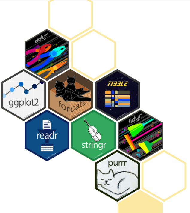
Figure 1.1: https://www.tidyverse.org/

1.17.1 and friends

• broom make outputs tidy
• lubridate working with dates
• readxl the readxl package contains the read_excel to read in .xls or .xlsx files
• knitr produce outputs such as HTML, PDF, Docs, PowerPoint, with Rmarkdown
• shiny build interactive web apps straight from R
• flexdashboard build dashboards with R
• furrr parallel mapping
• yardstick for model evaluation metrics

tidyverse_friends <- c('broom','lubridate','readxl','knitr','shiny','furrr','flexdashboard','yardstick')

install.packages(tidyverse_friends)

1.17.2 pipe opperator

The pipe %>% operator originates from the magrittr package. The pipe takes the information on the left and passes it to the information on the right:

f(x) is the same as x %>% f()

Notice how x gets piped into a function f

glimpse(my_dataframe)
#> Rows: 4
#> Columns: 7
#> $ list_of_ints          <int> 2, 4, 6, 8
#> $ list_of_strings       <chr> "Data", "Science", "is a", "blast!"
#> $ list_of_logicals      <lgl> TRUE, FALSE, TRUE, FALSE
#> $ list_of_mixed_type    <chr> "3.14", "1", "cat", "TRUE"
#> $ list_of_numbers       <dbl> 3.142857, 18.000000, 42.000000, 65.200000
#> $ list_of_sexes_factor  <fct> Male, Female, Female, Male
#> $ ordered_list_of_costs <ord> $0 - $100, $100 - $200, $200 - $300, $300 - $400

is the same as

my_dataframe %>%
 glimpse()
#> Rows: 4
#> Columns: 7
#> $ list_of_ints          <int> 2, 4, 6, 8
#> $ list_of_strings       <chr> "Data", "Science", "is a", "blast!"
#> $ list_of_logicals      <lgl> TRUE, FALSE, TRUE, FALSE
#> $ list_of_mixed_type    <chr> "3.14", "1", "cat", "TRUE"
#> $ list_of_numbers       <dbl> 3.142857, 18.000000, 42.000000, 65.200000
#> $ list_of_sexes_factor  <fct> Male, Female, Female, Male
#> $ ordered_list_of_costs <ord> $0 - $100, $100 - $200, $200 - $300, $300 - $400

Note that this pipe operation has become so popular in R version 4.1.0 now comes equipped with a pipe operator of it’s own:

1:10 |> mean()
#> [1] 5.5

\(~\)

---

\(~\)

1.17.3 Other Packages

Other packages we that will will make use of throughout the course of the text:

• devtools develop R packages

  • Note that devtools on Windows also requires Rtools https://cran.r-project.org/bin/windows/Rtools/

• arsenal compare dataframes ; create summary tables

• skimr automate Exploratory Data Analysis

• DataExplorer automate Exploratory Data Analysis

• rsq computes Adjusted R² for various model types

• RSQLite R package for interfacing with SQLite database

• dbplyr database back-end for dplyr

• plotly interactive HTML plots

• DT contains datatable function for interactive HTML datatable

• GGally contains ggcorr for correlation plots and ggpairs for other data-plots

• corrr correlation matrix as a data-frame

• AMR Principal Component Plots

• randomForest fit a Random Forest model

• caret (Classification And Regression Training) is a set of functions that attempt to streamline the process for creating predictive models.

• shiny Shiny is an R package that makes it easy to build interactive web apps straight from R.

• usethis usethis is a workflow package; it automates repetitive tasks that arise during project setup and development, both for R packages and non-package projects.

• testthat testthat is a package designed to assist with unit testing functions within packages.

• pkgdown pkgdown is designed to make it quick and easy to build a website for your package.

other_packages <- c('devtools','rsq','arsenal','skimr','DataExplorer',
                    'RSQLite','dbplyr','plotly','DT','GGally','corrr',
                    'AMR','caret','randomForest','shiny','usethis','testthat','pkgdown')

install.packages(other_packages)

\(~\)

---

\(~\)

1.18 Package Versions

We already mentioned that install.packages will update the package from CRAN:

install.packages( c( tidyverse_friends , other_packages ), repos = "http://cran.us.r-project.org")

We also use devtools to install the most-up-to-date package from github, for example:

devtools::install_github("tidyverse/tidyverse")

Here are the versions installed on this system, compare with your own:

as_tibble(installed.packages()) %>%
  select(Package, Version, Depends) %>% 
  filter(Package %in% c( c('tidyverse'),
         c('tibble','readr','dplyr','tidyr','stringr','purrr','ggplot2','forcats'),
           c( tidyverse_friends , other_packages )  )) %>%
  knitr::kable()

Package	Version	Depends
AMR	1.8.2	R (>= 3.0.0)
arsenal	3.6.3	R (>= 3.4.0), stats (>= 3.4.0)
broom	1.0.2	R (>= 3.1)
caret	6.0-93	ggplot2, lattice (>= 0.20), R (>= 3.2.0)
corrr	0.4.4	R (>= 3.4)
DataExplorer	0.8.2	R (>= 3.6)
dbplyr	2.2.1	R (>= 3.1)
dplyr	1.0.10	R (>= 3.4.0)
DT	0.26	NA
forcats	0.5.2	R (>= 3.4)
furrr	0.3.1	future (>= 1.25.0), R (>= 3.4.0)
GGally	2.1.2	R (>= 3.1), ggplot2 (>= 3.3.4)
ggplot2	3.4.0	R (>= 3.3)
knitr	1.41	R (>= 3.3.0)
lubridate	1.9.0	methods, timechange (>= 0.1.1), R (>= 3.2)
plotly	4.10.1.9000	R (>= 3.2.0), ggplot2 (>= 3.0.0)
purrr	1.0.0	R (>= 3.2.3)
randomForest	4.7-1.1	R (>= 4.1.0), stats
readr	2.1.3	R (>= 3.4)
readxl	1.4.1	R (>= 3.4)
rsq	2.5	NA
RSQLite	2.2.20	R (>= 3.1.0)
shiny	1.7.4	R (>= 3.0.2), methods
skimr	2.1.5	R (>= 3.1.2)
stringr	1.5.0	R (>= 3.3)
testthat	3.1.6	R (>= 3.1)
tibble	3.1.8	R (>= 3.1.0)
tidyr	1.2.1	R (>= 3.1)
tidyverse	1.3.2	R (>= 3.3)
yardstick	1.1.0	R (>= 3.4.0)

You can install specific versions of packages with: devtools::install_version("my.package.name", version = "0.9.1")

1.19 Details on this machine’s version of R

tibble::enframe(Sys.info()) %>%
  filter(name %in% c('sysname','release','version','machine')) %>%
  knitr::kable()

name	value
sysname	Windows
release	10 x64
version	build 22621
machine	x86-64

tibble::as_tibble(R.Version()) %>%
  pivot_longer(everything()) %>%
  knitr::kable()

name	value
platform	x86_64-w64-mingw32
arch	x86_64
os	mingw32
crt	ucrt
system	x86_64, mingw32
status
major	4
minor	2.2
year	2022
month	10
day	31
svn rev	83211
language	R
version.string	R version 4.2.2 (2022-10-31 ucrt)
nickname	Innocent and Trusting

1.19.1 sessionInfo

All the details about the current running session of R:

sessionInfo()
#> R version 4.2.2 (2022-10-31 ucrt)
#> Platform: x86_64-w64-mingw32/x64 (64-bit)
#> Running under: Windows 10 x64 (build 22621)
#> 
#> Matrix products: default
#> 
#> locale:
#> [1] LC_COLLATE=English_United States.utf8 
#> [2] LC_CTYPE=English_United States.utf8   
#> [3] LC_MONETARY=English_United States.utf8
#> [4] LC_NUMERIC=C                          
#> [5] LC_TIME=English_United States.utf8    
#> 
#> attached base packages:
#> [1] stats     graphics  grDevices utils     datasets  methods   base     
#> 
#> other attached packages:
#> [1] forcats_0.5.2   stringr_1.5.0   purrr_1.0.0     readr_2.1.3    
#> [5] tidyr_1.2.1     tibble_3.1.8    ggplot2_3.4.0   tidyverse_1.3.2
#> [9] dplyr_1.0.10   
#> 
#> loaded via a namespace (and not attached):
#>  [1] lubridate_1.9.0     assertthat_0.2.1    digest_0.6.31      
#>  [4] utf8_1.2.2          R6_2.5.1            cellranger_1.1.0   
#>  [7] backports_1.4.1     reprex_2.0.2        evaluate_0.19      
#> [10] httr_1.4.4          highr_0.10          pillar_1.8.1       
#> [13] rlang_1.0.6         googlesheets4_1.0.1 readxl_1.4.1       
#> [16] rstudioapi_0.14     jquerylib_0.1.4     rmarkdown_2.19     
#> [19] googledrive_2.0.0   munsell_0.5.0       broom_1.0.2        
#> [22] compiler_4.2.2      modelr_0.1.10       xfun_0.36          
#> [25] pkgconfig_2.0.3     htmltools_0.5.4     downlit_0.4.2      
#> [28] tidyselect_1.2.0    bookdown_0.31       codetools_0.2-18   
#> [31] fansi_1.0.3         crayon_1.5.2        tzdb_0.3.0         
#> [34] dbplyr_2.2.1        withr_2.5.0         grid_4.2.2         
#> [37] jsonlite_1.8.4      gtable_0.3.1        lifecycle_1.0.3    
#> [40] DBI_1.1.3           magrittr_2.0.3      scales_1.2.1       
#> [43] cli_3.5.0           stringi_1.7.8       cachem_1.0.6       
#> [46] fs_1.5.2            xml2_1.3.3          bslib_0.4.2        
#> [49] ellipsis_0.3.2      generics_0.1.3      vctrs_0.5.1        
#> [52] tools_4.2.2         glue_1.6.2          hms_1.1.2          
#> [55] fastmap_1.1.0       yaml_2.3.6          timechange_0.1.1   
#> [58] colorspace_2.0-3    gargle_1.2.1        rvest_1.0.3        
#> [61] memoise_2.0.1       knitr_1.41          haven_2.5.1        
#> [64] sass_0.4.4