9 Functional dbplyr, purrr, and furrr
library('tidyverse')
#> ── Attaching packages ─────────────────────────────────────── tidyverse 1.3.2 ──
#> ✔ ggplot2 3.4.0      ✔ purrr   1.0.0
#> ✔ tibble  3.1.8      ✔ dplyr   1.0.10
#> ✔ tidyr   1.2.1      ✔ stringr 1.5.0
#> ✔ readr   2.1.3      ✔ forcats 0.5.2
#> ── Conflicts ────────────────────────────────────────── tidyverse_conflicts() ──
#> ✖ dplyr::filter() masks stats::filter()
#> ✖ dplyr::lag()    masks stats::lag()

source('Functions/connect_help.R')
#> Warning: `src_sqlite()` was deprecated in dplyr 1.0.0.
#> ℹ Please use `tbl()` directly with a database connection
9.0.0.1 source current target
source('Week_4/FEATURES/Store_TARGET_DM2.R')
#> Joining, by = "yr_range"
#> Joining, by = "SEQN"
#> Joining, by = "SEQN"
9.0.0.2 source current features
source('Week_4/FEATURES/Store_DEMO.R')
#> Joining, by = "SEQN"
#> Joining, by = "SEQN"
#> Joining, by = "SEQN"
#> Joining, by = "SEQN"
#> Joining, by = "SEQN"
#> Joining, by = "SEQN"
#> Joining, by = "SEQN"
#> Joining, by = "SEQN"
source('Week_4/FEATURES/Store_EXAM.R')
#> Joining, by = c("SEQN", "yr_range")
#> Joining, by = c("SEQN", "yr_range")
source('Week_4/FEATURES/Store_LABS.R')
#> Joining, by = c("SEQN", "yr_range")
#> Joining, by = c("SEQN", "yr_range")
#> Joining, by = c("SEQN", "yr_range")
#> Joining, by = c("SEQN", "yr_range")
#> Joining, by = c("SEQN", "yr_range")
#> Warning: Expected 2 pieces. Missing pieces filled with `NA` in 30 rows [1, 2, 3,
#> 4, 5, 6, 7, 8, 9, 10, 11, 12, 13, 14, 16, 17, 18, 19, 20, 21, ...].
9.0.1 A_DATA_TBL_2
We want to make a new Analytic data-set from additional features that have been developed. We might begin to cultivate a Feature Store which might comprise of either code or data to replicate features.
A_DATA_TBL_2 <- DEMO %>%
  select(SEQN) %>%
  left_join(OUTCOME_TBL) %>%
  left_join(DEMO_FEATURES) %>%
  left_join(EXAM_TBL) %>%
  left_join(LABS_TBL)
#> Joining, by = "SEQN"
#> Joining, by = "SEQN"
#> Joining, by = "SEQN"
#> Joining, by = c("SEQN", "yr_range")
Get the dimension from a connection
# number of rows
Tot_N_Rows <- (A_DATA_TBL_2 %>%
  tally() %>%
  collect())$n

Tot_N_Rows
#> [1] 101316

# number of columns
A_DATA_TBL_2 %>%
  colnames() %>%
  length()
#> [1] 133
#look at the data-set
A_DATA_TBL_2 %>%
  head()
#> # Source:   SQL [6 x 133]
#> # Database: sqlite 3.40.0 [C:\Users\jkyle\Documents\GitHub\Jeff_Data_Wrangling\DATA\sql_db\NHANES_DB.db]
#>    SEQN DIABE…¹ AGE_A…²   Age Gender Race  USAF  Birth…³ Grade…⁴ Grade…⁵ Marit…⁶
#>   <dbl>   <dbl> <lgl>   <dbl> <chr>  <chr> <chr> <chr>   <chr>   <chr>   <chr>
#> 1     1       0 NA          2 Female Black <NA>  USA     <NA>    <NA>    <NA>
#> 2     2       0 NA         77 Male   White Yes   USA     <NA>    Colleg… <NA>
#> 3     3       0 NA         10 Female White <NA>  <NA>    3rd gr… <NA>    <NA>
#> 4     4       0 NA          1 Male   Black <NA>  USA     <NA>    <NA>    <NA>
#> 5     5       0 NA         49 Male   White Yes   USA     <NA>    Colleg… Married
#> 6     6       0 NA         19 Female Other No    USA     More t… <NA>    Never …
#> # … with 122 more variables: Pregnant <chr>, Household_Icome <lgl>,
#> #   Family_Income <lgl>, Poverty_Income_Ratio <dbl>, yr_range <chr>,
#> #   PEASCST1 <dbl>, PEASCTM1 <dbl>, PEASCCT1 <dbl>, BPXCHR <dbl>,
#> #   BPQ150A <dbl>, BPQ150B <dbl>, BPQ150C <dbl>, BPQ150D <dbl>, BPAARM <dbl>,
#> #   BPACSZ <dbl>, BPXPLS <dbl>, BPXDB <dbl>, BPXPULS <dbl>, BPXPTY <dbl>,
#> #   BPXML1 <dbl>, BPXSY1 <dbl>, BPXDI1 <dbl>, BPAEN1 <dbl>, BPXSY2 <dbl>,
#> #   BPXDI2 <dbl>, BPAEN2 <dbl>, BPXSY3 <dbl>, BPXDI3 <dbl>, BPAEN3 <dbl>, …
\(~\)
\(~\)
9.1 Determining Categorical and Continuous Features
Not_features <- c('SEQN', 'DIABETES', 'AGE_AT_DIAG_DM2')
All_featres <- setdiff(colnames(A_DATA_TBL_2), Not_features)
N_levels_features <- A_DATA_TBL_2 %>%
  collect( ) %>% # note this collects all the data
  select(- all_of(Not_features)) %>%
  summarise_at(vars(all_of(All_featres)), ~ n_distinct(.x))

N_levels_features %>%
  head()
#> # A tibble: 1 × 130
#>     Age Gender  Race  USAF Birth_Country Grade…¹ Grade…² Marit…³ Pregn…⁴ House…⁵
#>   <int>  <int> <int> <int>         <int>   <int>   <int>   <int>   <int>   <int>
#> 1    86      2     5     3             3      21       6       7       3      15
#> # … with 120 more variables: Family_Income <int>, Poverty_Income_Ratio <int>,
#> #   yr_range <int>, PEASCST1 <int>, PEASCTM1 <int>, PEASCCT1 <int>,
#> #   BPXCHR <int>, BPQ150A <int>, BPQ150B <int>, BPQ150C <int>, BPQ150D <int>,
#> #   BPAARM <int>, BPACSZ <int>, BPXPLS <int>, BPXDB <int>, BPXPULS <int>,
#> #   BPXPTY <int>, BPXML1 <int>, BPXSY1 <int>, BPXDI1 <int>, BPAEN1 <int>,
#> #   BPXSY2 <int>, BPXDI2 <int>, BPAEN2 <int>, BPXSY3 <int>, BPXDI3 <int>,
#> #   BPAEN3 <int>, BPXSY4 <int>, BPXDI4 <int>, BPAEN4 <int>, BPXSAR <int>, …
N_levels_features %>%
  pivot_longer( cols = all_of(All_featres), values_to = "N_Distinct_Values")
#> # A tibble: 130 × 2
#>   name          N_Distinct_Values
#>   <chr>                     <int>
#> 1 Age                          86
#> 2 Gender                        2
#> 3 Race                          5
#> 4 USAF                          3
#> 5 Birth_Country                 3
#> 6 Grade_Level                  21
#> # … with 124 more rows
N_levels_features %>%
  pivot_longer( cols = all_of(All_featres), values_to = "N_Distinct_Values") %>%
  mutate(Fearure = reorder(name, -N_Distinct_Values)) %>%
  mutate(Percentage_Distinct_Features = N_Distinct_Values/Tot_N_Rows ) %>%
  ggplot(aes(x= Fearure, y=Percentage_Distinct_Features , color=Fearure)) +
  geom_bar(stat = "identity") +
  coord_flip() +
theme(legend.position = "none") 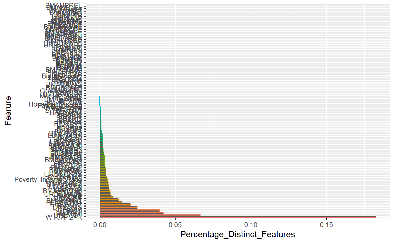
Figure 9.1: Count of Distinct Number of Values Per Feature
N_levels_features %>%
  pivot_longer( cols = all_of(All_featres), values_to = "N_Distinct_Values") %>%
  arrange(N_Distinct_Values) %>%
  filter(15 <  N_Distinct_Values &  N_Distinct_Values < 70)
#> # A tibble: 8 × 2
#>   name        N_Distinct_Values
#>   <chr>                   <int>
#> 1 Grade_Level                21
#> 2 PHAFSTHR                   45
#> 3 BPXML1                     48
#> 4 PHAFSTMN                   61
#> 5 BPXDI4                     65
#> 6 BPXPLS                     67
#> # … with 2 more rows
categorical_features <- (N_levels_features %>%
  pivot_longer( cols = all_of(All_featres), values_to = "N_Distinct_Values") %>%
  arrange(N_Distinct_Values) %>%
  filter(N_Distinct_Values <= 25))$name

categorical_features
#>  [1] "BMAUPREL"        "BMAUPLEL"        "Gender"          "BMIHEAD"
#>  [5] "BMILEG"          "BMICALF"         "BMIARML"         "BMIARMC"
#>  [9] "BMIWAIST"        "BMITHICR"        "BMAUREXT"        "BMAULEXT"
#> [13] "BMALOREX"        "BMALORKN"        "BMALLKNE"        "BMDRECUF"
#> [17] "BMDSUBF"         "BMDTHICF"        "BMDLEGF"         "BMDARMLF"
#> [21] "BMDCALFF"        "BMIHIP"          "USAF"            "Birth_Country"
#> [25] "Pregnant"        "BPQ150A"         "BPQ150B"         "BPQ150C"
#> [29] "BPQ150D"         "BPXPULS"         "BPXPTY"          "BPAEN1"
#> [33] "BPAEN2"          "BPAEN3"          "BPAEN4"          "BMIRECUM"
#> [37] "BMIHT"           "BMITRI"          "BMISUB"          "BMAAMP"
#> [41] "BMALLEXT"        "URDUMALC"        "URDUCRLC"        "LBDINLC"
#> [45] "PEASCST1"        "BPAARM"          "BMAEXSTS"        "BMIWT"
#> [49] "URXPREG"         "Race"            "BMDSTATS"        "BMDBMIC"
#> [53] "Grade_Range"     "BPACSZ"          "BMDSADCM"        "Marital_Status"
#> [57] "yr_range"        "BMAEXCMT"        "BPXDB"           "Household_Icome"
#> [61] "Family_Income"   "PEASCCT1"        "Grade_Level"
Currently, there are 63 and
numeric_features <- (N_levels_features %>%
  pivot_longer( cols = all_of(All_featres), values_to = "N_Distinct_Values") %>%
  arrange(N_Distinct_Values) %>%
  filter(N_Distinct_Values > 25))$name

numeric_features
#>  [1] "PHAFSTHR"             "BPXML1"               "PHAFSTMN"
#>  [4] "BPXDI4"               "BPXPLS"               "BPXDI1"
#>  [7] "BPXDI3"               "BPXDI2"               "BPXSY4"
#> [10] "BPXCHR"               "BPXSY3"               "Age"
#> [13] "BPXSY2"               "BPXSY1"               "BPXDAR"
#> [16] "BMXHEAD"              "LBDHDD"               "LBDHDDSI"
#> [19] "BPXSAR"               "LBXAPB"               "LBDAPBSI"
#> [22] "LBDLDLM"              "LBDLDMSI"             "LBDLDLN"
#> [25] "LBDLDNSI"             "BMXSAD3"              "BMXSAD4"
#> [28] "LBDLDL"               "LBDLDLSI"             "BMXSAD1"
#> [31] "BMXSAD2"              "BMDAVSAD"             "BMXLEG"
#> [34] "LBXTC"                "LBDTCSI"              "LBXGLU"
#> [37] "BMXCALF"              "BMXARML"              "BMXSUB"
#> [40] "URXUCR2"              "URDUCR2S"             "BMXTRI"
#> [43] "BMXARMC"              "Poverty_Income_Ratio" "BMAEXLEN"
#> [46] "URXUCR"               "BMXTHICR"             "LBDGLUSI"
#> [49] "LBXTR"                "LBDTRSI"              "BMXRECUM"
#> [52] "URXUMA2"              "URDUMA2S"             "BMXHIP"
#> [55] "URXCRS"               "BMXHT"                "BMXWAIST"
#> [58] "PEASCTM1"             "URDACT2"              "BMXWT"
#> [61] "URXUMA"               "URXUMS"               "LBXIN"
#> [64] "LBDINSI"              "BMXBMI"               "URDACT"
#> [67] "WTSAF2YR"
we have 67 numeric features to analyze.
We can save both of these lists into an new object:
FEATURE_TYPE <- new.env()
FEATURE_TYPE$numeric_features <- numeric_features
FEATURE_TYPE$categorical_features <- categorical_features
FEATURE_TYPE$Not_features <- Not_features
We can still access the information, however, now it is grouped together:
FEATURE_TYPE$categorical_features
#>  [1] "BMAUPREL"        "BMAUPLEL"        "Gender"          "BMIHEAD"
#>  [5] "BMILEG"          "BMICALF"         "BMIARML"         "BMIARMC"
#>  [9] "BMIWAIST"        "BMITHICR"        "BMAUREXT"        "BMAULEXT"
#> [13] "BMALOREX"        "BMALORKN"        "BMALLKNE"        "BMDRECUF"
#> [17] "BMDSUBF"         "BMDTHICF"        "BMDLEGF"         "BMDARMLF"
#> [21] "BMDCALFF"        "BMIHIP"          "USAF"            "Birth_Country"
#> [25] "Pregnant"        "BPQ150A"         "BPQ150B"         "BPQ150C"
#> [29] "BPQ150D"         "BPXPULS"         "BPXPTY"          "BPAEN1"
#> [33] "BPAEN2"          "BPAEN3"          "BPAEN4"          "BMIRECUM"
#> [37] "BMIHT"           "BMITRI"          "BMISUB"          "BMAAMP"
#> [41] "BMALLEXT"        "URDUMALC"        "URDUCRLC"        "LBDINLC"
#> [45] "PEASCST1"        "BPAARM"          "BMAEXSTS"        "BMIWT"
#> [49] "URXPREG"         "Race"            "BMDSTATS"        "BMDBMIC"
#> [53] "Grade_Range"     "BPACSZ"          "BMDSADCM"        "Marital_Status"
#> [57] "yr_range"        "BMAEXCMT"        "BPXDB"           "Household_Icome"
#> [61] "Family_Income"   "PEASCCT1"        "Grade_Level"
FEATURE_TYPE[['numeric_features']]
#>  [1] "PHAFSTHR"             "BPXML1"               "PHAFSTMN"
#>  [4] "BPXDI4"               "BPXPLS"               "BPXDI1"
#>  [7] "BPXDI3"               "BPXDI2"               "BPXSY4"
#> [10] "BPXCHR"               "BPXSY3"               "Age"
#> [13] "BPXSY2"               "BPXSY1"               "BPXDAR"
#> [16] "BMXHEAD"              "LBDHDD"               "LBDHDDSI"
#> [19] "BPXSAR"               "LBXAPB"               "LBDAPBSI"
#> [22] "LBDLDLM"              "LBDLDMSI"             "LBDLDLN"
#> [25] "LBDLDNSI"             "BMXSAD3"              "BMXSAD4"
#> [28] "LBDLDL"               "LBDLDLSI"             "BMXSAD1"
#> [31] "BMXSAD2"              "BMDAVSAD"             "BMXLEG"
#> [34] "LBXTC"                "LBDTCSI"              "LBXGLU"
#> [37] "BMXCALF"              "BMXARML"              "BMXSUB"
#> [40] "URXUCR2"              "URDUCR2S"             "BMXTRI"
#> [43] "BMXARMC"              "Poverty_Income_Ratio" "BMAEXLEN"
#> [46] "URXUCR"               "BMXTHICR"             "LBDGLUSI"
#> [49] "LBXTR"                "LBDTRSI"              "BMXRECUM"
#> [52] "URXUMA2"              "URDUMA2S"             "BMXHIP"
#> [55] "URXCRS"               "BMXHT"                "BMXWAIST"
#> [58] "PEASCTM1"             "URDACT2"              "BMXWT"
#> [61] "URXUMA"               "URXUMS"               "LBXIN"
#> [64] "LBDINSI"              "BMXBMI"               "URDACT"
#> [67] "WTSAF2YR"
9.1.1 distinct_N_levels_per_cols
Below is a helper function for the count of distinct column entries in a table per the first sample_n records queried
distinct_N_levels_per_cols <- function(data, sample_n = 2000){

  data.colnames <- colnames(data)

  N_levels_features <- data %>%
    collect( n = sample_n ) %>% # note this collects sample_n rows of data
    summarise_at(all_of(data.colnames), ~ n_distinct(.x)) %>%
    pivot_longer( cols = all_of(data.colnames), values_to = "N_Distinct_Values")

  plot <- N_levels_features %>%
  mutate(Fearure = reorder(name, -N_Distinct_Values)) %>%
  mutate(Percentage_Distinct_Features = N_Distinct_Values/sample_n ) %>%
  ggplot(aes(x= Fearure, y=Percentage_Distinct_Features , color=Fearure)) +
  geom_bar(stat = "identity") +
  coord_flip() +
  labs(title ="Percentage of Distinct Entries Per Column",
       subtitle = paste0("Per Sample of ", sample_n, " records")) +
  theme(legend.position = "none")

  return( list( data = N_levels_features,
                plot = plot))
}
distinct_N_levels_per_cols(A_DATA_TBL_2, 3241)
#> Warning: Using `all_of()` outside of a selecting function was deprecated in tidyselect
#> 1.2.0.
#> ℹ See details at
#>   <https://tidyselect.r-lib.org/reference/faq-selection-context.html>
#> $data
#> # A tibble: 133 × 2
#>   name            N_Distinct_Values
#>   <chr>                       <int>
#> 1 SEQN                         3241
#> 2 DIABETES                        3
#> 3 AGE_AT_DIAG_DM2                65
#> 4 Age                            86
#> 5 Gender                          2
#> 6 Race                            5
#> # … with 127 more rows
#>
#> $plot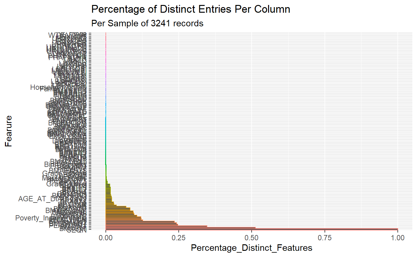
Figure 9.2: Count of Distinct Number of Values Per Feature per first 3,241 records
9.2 Categorical Features
Recall, we normally want to review categorical data by looking at frequency counts:
A_DATA_TBL_2 %>%
  select(DIABETES, Gender) %>%
  collect() %>%
  group_by(DIABETES, Gender) %>%
  tally() %>%
  pivot_wider(names_from = Gender, values_from = n)
#> # A tibble: 3 × 3
#> # Groups:   DIABETES [3]
#>   DIABETES Female  Male
#>      <dbl>  <int> <int>
#> 1        0  45188 43552
#> 2        1   3371  3436
#> 3       NA   2864  2905
A_DATA_TBL_2 %>%
  select(DIABETES, Race) %>%
  collect() %>%
  group_by(DIABETES, Race) %>%
  tally() %>%
  ungroup() %>%
  pivot_wider(names_from = Race, values_from = n)
#> # A tibble: 3 × 6
#>   DIABETES Black `Mexican American` Other `Other Hispanic` White
#>      <dbl> <int>              <int> <int>            <int> <int>
#> 1        0 20692              19426  8376             7201 33045
#> 2        1  1823               1373   611              592  2408
#> 3       NA  1129               1650   510              501  1979
9.2.1 Count_Query function
So to functionalize this process we create the following:
Count_Query <- function(my_feature){
  enquo_feature <- enquo(my_feature)

 tmp <- A_DATA_TBL_2 %>%
    select(DIABETES, !!enquo_feature) %>%
    collect() %>%
    group_by(DIABETES, !!enquo_feature) %>%
    tally() %>%
    ungroup() %>%
    pivot_wider(names_from = !!enquo_feature, values_from = n)

return(tmp)
}
What is enquo?
enquo() and enquos() delay the execution of one or several function arguments. enquo() returns a single quoted expression, which is like a blueprint for the delayed computation. enquos() returns a list of such quoted expressions. We can resolve an enquo with !!.
Count_Query(Grade_Level)
#> # A tibble: 3 × 22
#> DIABETES `10th grade` 11th g…¹ 12th …² 1st g…³ 2nd g…⁴ 3rd g…⁵ 4th g…⁶ 5th g…⁷
#> <dbl> <int> <int> <int> <int> <int> <int> <int> <int>
#> 1 0 2177 2146 438 2126 2102 2031 2036 2110
#> 2 1 11 12 NA 6 4 6 6 9
#> 3 NA 9 8 2 2 1 6 12 10
#> # … with 13 more variables: `6th grade` <int>, `7th grade` <int>,
#> # `8th grade` <int>, `9th grade` <int>, `Don't Know` <int>,
#> # `GED or equivalent` <int>, `High school graduate` <int>,
#> # `Less than 5th grade` <int>, `Less than 9th grade` <int>,
#> # `More than high school` <int>, `Never attended / kindergarten only` <int>,
#> # Refused <int>, `NA` <int>, and abbreviated variable names ¹`11th grade`,
#> # ²`12th grade, no diploma`, ³`1st grade`, ⁴`2nd grade`, ⁵`3rd grade`, …
Count_Query(Household_Icome)
#> # A tibble: 3 × 16
#> DIABETES $ 0 to $ 4,…¹ $ 5,0…² $10,0…³ $100,…⁴ $15,0…⁵ $20,0…⁶ $20,0…⁷ $25,0…⁸
#> <dbl> <int> <int> <int> <int> <int> <int> <int> <int>
#> 1 0 1349 2012 3169 8226 3427 1781 3902 5994
#> 2 1 96 268 452 460 375 194 417 526
#> 3 NA 118 150 236 440 254 119 277 399
#> # … with 7 more variables: `$35,000 to $44,999` <int>,
#> # `$45,000 to $54,999` <int>, `$55,000 to $64,999` <int>,
#> # `$65,000 to $74,999` <int>, `$75,000 to $99,999` <int>,
#> # `Under $20,000` <int>, `NA` <int>, and abbreviated variable names
#> # ¹`$ 0 to $ 4,999`, ²`$ 5,000 to $ 9,999`, ³`$10,000 to $14,999`,
#> # ⁴`$100,000 and Over`, ⁵`$15,000 to $19,999`, ⁶`$20,000 and Over`,
#> # ⁷`$20,000 to $24,999`, ⁸`$25,000 to $34,999`9.2.2 Graphing Helpers
We can also make a function out of the chi-square mosaic plot:
plot_chi_square_residuals <- function(my_feature){
  enquo_feature <- enquo(my_feature)

  plot <- A_DATA_TBL_2 %>%
    select( !!enquo_feature, DIABETES) %>%
    collect() %>%
    table() %>%
    vcd::mosaic(gp = vcd::shading_max)

  return(plot)
}
plot_chi_square_residuals(Grade_Level)
#>                                    DIABETES    0    1
#> Grade_Level
#> 10th grade                                  2177   11
#> 11th grade                                  2146   12
#> 12th grade, no diploma                       438    0
#> 1st grade                                   2126    6
#> 2nd grade                                   2102    4
#> 3rd grade                                   2031    6
#> 4th grade                                   2036    6
#> 5th grade                                   2110    9
#> 6th grade                                   2219   14
#> 7th grade                                   2178    8
#> 8th grade                                   2292   11
#> 9th grade                                   2195   18
#> Don't Know                                     9    0
#> GED or equivalent                            115    0
#> High school graduate                        1422    9
#> Less than 5th grade                           26    0
#> Less than 9th grade                          277    1
#> More than high school                        980    6
#> Never attended / kindergarten only          2362    5
#> Refused                                        2    0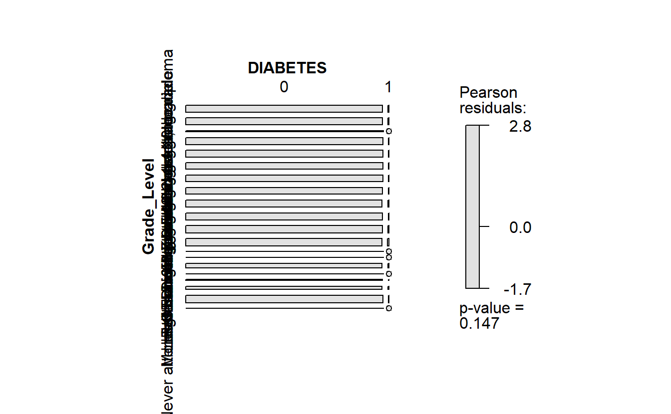
(#fig:4-1-chi-square-grade-level )Chi-Square residuals - Grade Level by Diabetes
Or a function to help us with bar graphs:
plot_cat_bar_graph <- function(my_feature){
  enquo_feature <- enquo(my_feature)

  plot <- A_DATA_TBL_2 %>%
    select(DIABETES, !!enquo_feature) %>%
    collect() %>%
    ggplot(aes(y= !!enquo_feature, fill= as.factor(DIABETES) )) +
    geom_bar(position = position_dodge(width = NULL))

  return(plot)
}
plot_cat_bar_graph(Grade_Level)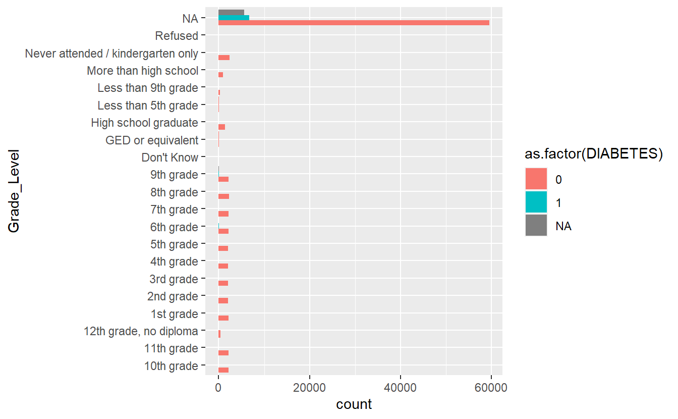
Figure 9.3: Bar Plot Grade Level by Diabetic Status
9.2.2.1 Combine functions to create new functions
We can combine functions:
cat_feature_explore <- function(my_feature){
  enquo_feature <- enquo(my_feature)


  return(list(Count_Query = Count_Query(!!enquo_feature),
              plot_chi_square_residuals = plot_chi_square_residuals(!!enquo_feature),
              plot_cat_bar_graph_y = plot_cat_bar_graph(!!enquo_feature)
              )
         )
}
cat_feature_explore(Gender)
#> $Count_Query
#> # A tibble: 3 × 3
#>   DIABETES Female  Male
#>      <dbl>  <int> <int>
#> 1        0  45188 43552
#> 2        1   3371  3436
#> 3       NA   2864  2905
#>
#> $plot_chi_square_residuals
#>        DIABETES     0     1
#> Gender
#> Female          45188  3371
#> Male            43552  3436
#>
#> $plot_cat_bar_graph_y
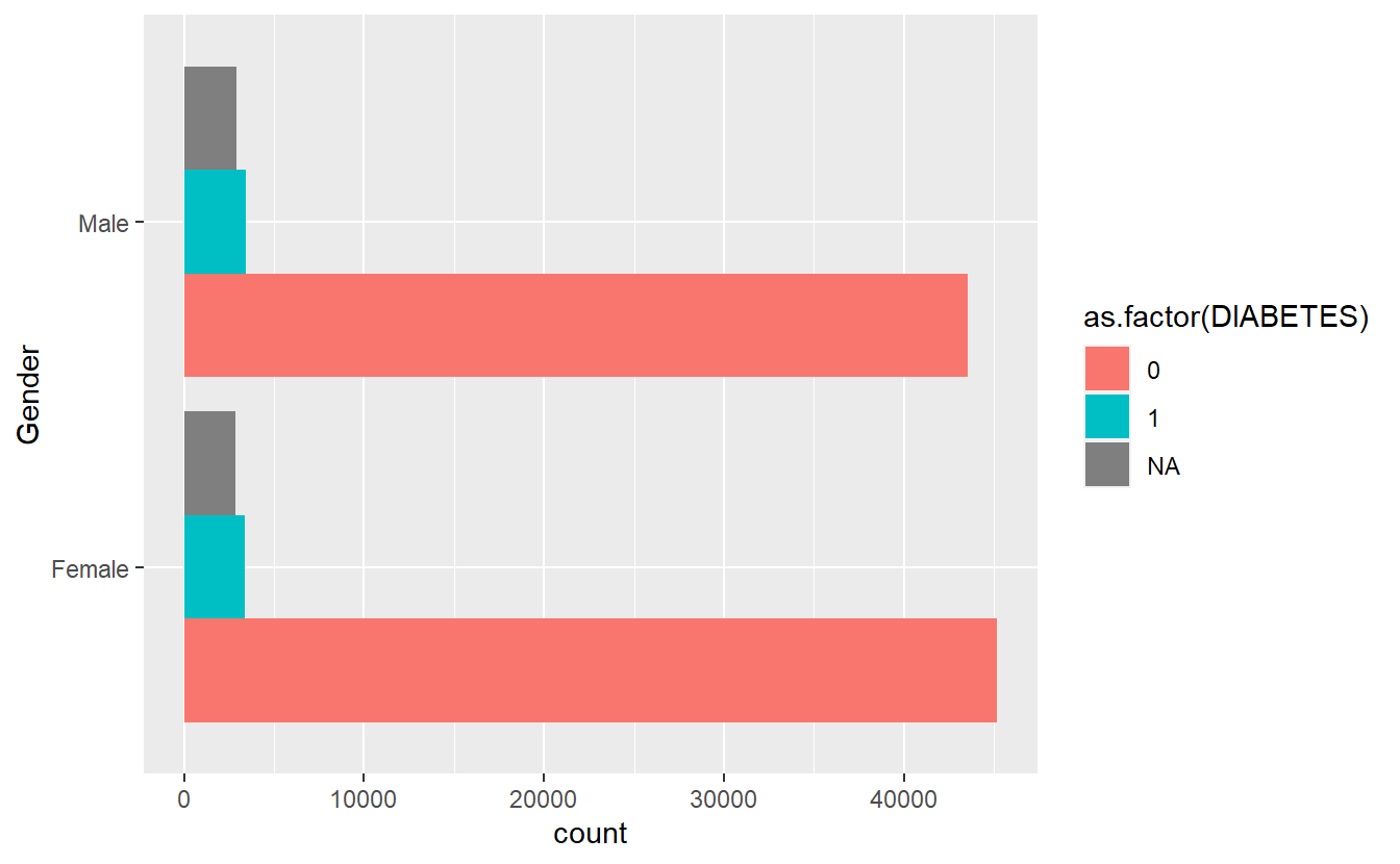
Figure 9.4: Combine Plots Gender
Note if we only want the graph from plot_cat_bar_graph plot we defined we can access it from plot_cat_bar_graph_y (or what ever we want to call it) this defined list:
cat_feature_explore(Gender)$plot_cat_bar_graph_y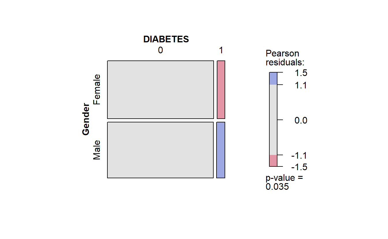

(#fig:4-1-combine-plot-plot_cat_bar_graph)Extract Bar Graph from Combined Function
toc <- Sys.time()

cat_feature_explore(Race)
#> $Count_Query
#> # A tibble: 3 × 6
#>   DIABETES Black `Mexican American` Other `Other Hispanic` White
#>      <dbl> <int>              <int> <int>            <int> <int>
#> 1        0 20692              19426  8376             7201 33045
#> 2        1  1823               1373   611              592  2408
#> 3       NA  1129               1650   510              501  1979
#>
#> $plot_chi_square_residuals
#>                  DIABETES     0     1
#> Race
#> Black                     20692  1823
#> Mexican American          19426  1373
#> Other                      8376   611
#> Other Hispanic             7201   592
#> White                     33045  2408
#>
#> $plot_cat_bar_graph_y

tic <- Sys.time()

time.cat_fun1.Race <- difftime(tic,toc,'secs')

time.cat_fun1.Race
#> Time difference of 13.17702 secs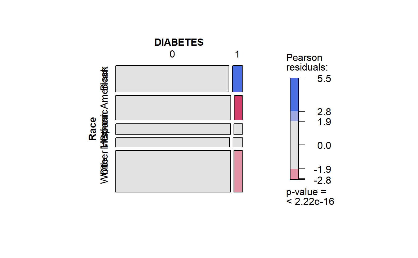

Figure 9.5: running cat_feature_explore on Race
9.2.2.2 Rewrite functions to gain speed-ups
We can better optimize this function if we collect the data one time instead of three:
cat_feature_explore <- function(my_feature){

  enquo_feature <- enquo(my_feature)

  tmp <- A_DATA_TBL_2 %>%
    select(DIABETES, !!enquo_feature) %>%
    collect()

   table1 <- table(tmp)

   plot_chi_square_residuals <-  vcd::mosaic(table1, gp = vcd::shading_max)

   plot_cat_bar_graph <- tmp %>%
    ggplot(aes(y= !!enquo_feature, fill= as.factor(DIABETES) )) +
    geom_bar(position = position_dodge(width = NULL))

   return( list(Frequency_Table = table1,
                plot_chi_square_residuals = plot_chi_square_residuals,
                plot_cat_bar_graph = plot_cat_bar_graph))

}
So now we test our function:
toc <- Sys.time()

cat_feature_explore(Race)
#> $Frequency_Table
#>         Race
#> DIABETES Black Mexican American Other Other Hispanic White
#>        0 20692            19426  8376           7201 33045
#>        1  1823             1373   611            592  2408
#>
#> $plot_chi_square_residuals
#>          Race Black Mexican American Other Other Hispanic White
#> DIABETES
#> 0             20692            19426  8376           7201 33045
#> 1              1823             1373   611            592  2408
#>
#> $plot_cat_bar_graph

tic <- Sys.time()

time.cat_fun2.Race <- difftime(tic,toc,'secs')

time.cat_fun2.Race
#> Time difference of 4.800569 secs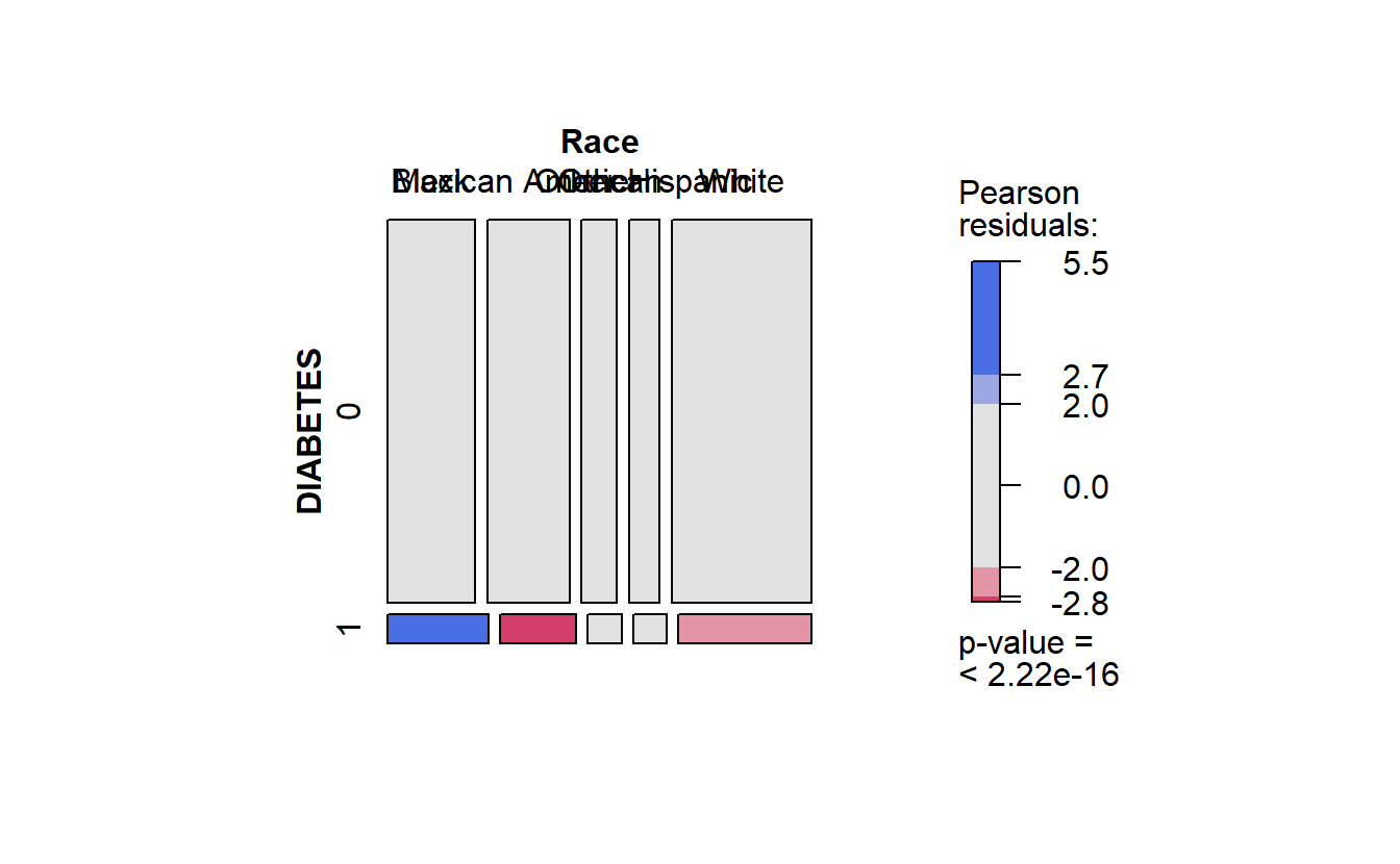
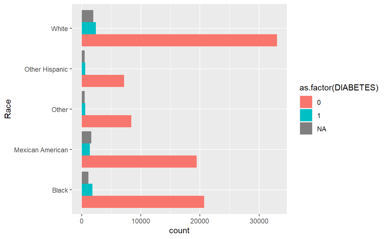
Figure 9.6: running faster cat_feature_explore on Race
Note if we only want the mosaic plot we defined in the plot_chi_square_residuals we can access it from this defined list:
cat_feature_explore(Race)$plot_chi_square_residuals
#>          Race Black Mexican American Other Other Hispanic White
#> DIABETES
#> 0             20692            19426  8376           7201 33045
#> 1              1823             1373   611            592  2408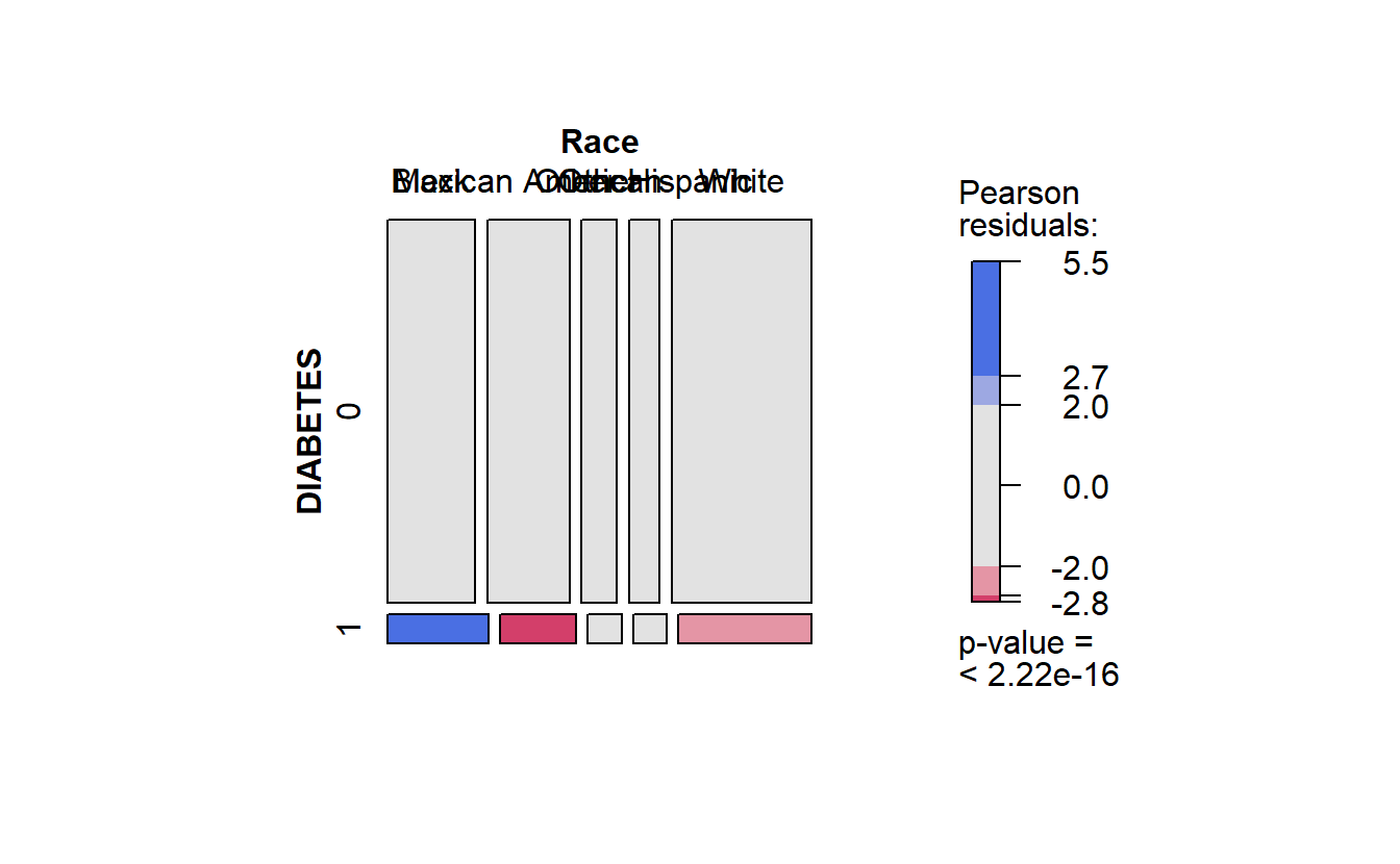
Figure 9.7: faster Race residuals
Recall in the mosaic plot that
- Blue indicates that the observed value is higher than the expected value if the data were random.
- Red color specifies that the observed value is lower than the expected value if the data were random.
Thus we already know that African Americans are more likely to have diabetes than White Americans.
Speed-Up Note the changes we made resulted in the function running
as.numeric(time.cat_fun1.Race)/as.numeric(time.cat_fun2.Race)
#> [1] 2.744888
times faster!
\(~\)
\(~\)
9.3 Additional Programming Refrences
- https://dplyr.tidyverse.org/reference/tidyeval.html
- https://dplyr.tidyverse.org/articles/programming.html
- https://tidyeval.tidyverse.org/dplyr.html#patterns-for-single-arguments
\(~\)
\(~\)
9.4 Continuous Features
Previously we had the following algorithm for a t-test:
## DONT RUN
{
DM2.Age <- (A_DATA %>%
  filter(DIABETES == 1))$Age

Non_DM2.Age <- (A_DATA %>%
  filter(DIABETES == 0))$Age

t_test.Age.Non_Dm2.DM2 <- t.test(Non_DM2.Age, DM2.Age,
                                 alternative = 'two.sided',
                                 conf.level = 0.95)

tibble_t_test.Age.Non_Dm2.DM2 <- broom::tidy(t_test.Age.Non_Dm2.DM2) %>%
  mutate(dist_1 = "Non_DM2.Age") %>%
  mutate(dist_2 = "DM2.Age")
}
That process was for one t.test, for one continuous feature, Age.
We might want to functionalize the process of computing t-tests for other similar analytic data-sets, like the one we are currently working with.
Developing such functions or wrappers may take time and skill but over-time you will come to rely on a personal library of functions you develop or work with to iterate on projects faster. These functions might start in your personal library and eventually move into a team Git where you or other members of your team can manage their development.
For instance, upon inspection, we notice that t.test requires similar information to ks.test. It would make sense to bundle two tests together and save us some time later on.
9.4.1 t-test / ks-test wrapper function
In the function wrapper.t_ks_test below takes in:
dfa tibble - data-frame or connection-
factora categorical variable in df- Note in SQLlite there is no factor type but the user thinks of this variable as a factor
factor_level- sets the “first” class in a one-versus-restt.testandks.testanalysiscontinuous_featurerepresented by a character string of the feature name to performt.testandks.testonverbosewas useful in creating the function to identify variables causing errors, and create output for those types of cases.
wrapper.t_ks_test <- function(df, factor, factor_level,  continuous_feature, verbose = FALSE){

  if(verbose == TRUE){
    cat(paste0('\n','Now on Feature ',continuous_feature,' \n'))
  }

  factor_enquo <- enquo(factor)

  data.local <- df %>%
    select(!! factor_enquo, matches(continuous_feature)) %>%
    collect()

  X <- data.local %>%
    filter(!! factor_enquo == factor_level)

  Y <- data.local %>%
    filter(!(!! factor_enquo == factor_level))

  x <- unlist(X[,continuous_feature])
  y <- unlist(Y[,continuous_feature])

  sd_x <- sd(x, na.rm=TRUE)
  sd_y <- sd(y, na.rm=TRUE)

  if(sum(!is.na(x)) < 3 | sum(!is.na(y)) < 3 | is.na(sd_x) | is.na(sd_y) | sd_x == 0 | sd_y == 0){

    bad_return <- tibble(mean_diff_est = mean(x , na.rm=TRUE) - mean(y , na.rm=TRUE),
                         N_Target = sum(!is.na(x)),
                         mean_Target = mean(x , na.rm=TRUE),
                         sd_Target = sd_x,
                         N_Control = sum(!is.na(y)),
                         mean_Control = mean(y , na.rm=TRUE),
                         sd_Control = sd_y,
                         statistic = NA,
                         ttest.pvalue = NA,
                         kstest.pvalue = NA,
                         parameter = NA,
                         conf.low = NA,
                         conf.high = NA,
                         method = "Either Target or Control has fewer than 3 results",
                         alternative = paste0(continuous_feature, " Might be constant"),
                         Feature = continuous_feature) %>%
      select(Feature, mean_diff_est, ttest.pvalue, mean_Target, mean_Control, kstest.pvalue, N_Target, N_Control, conf.low, conf.high, statistic, sd_Target, sd_Control, parameter, method, alternative)
    return(bad_return)

  }

  ttest_return <- t.test(x,y)

  ks.test.pvalue <- suppressWarnings(ks.test(x,y)$p.value)

  result_row <- broom::tidy(ttest_return)

  result_row <- result_row %>%
    mutate(Feature = continuous_feature) %>%
    rename(mean_diff_est = estimate) %>%
    mutate(N_Target = sum(!is.na(x))) %>%
    mutate(N_Control = sum(!is.na(y))) %>%
    rename(mean_Target = estimate1) %>%
    rename(mean_Control = estimate2) %>%
    rename(ttest.pvalue = p.value) %>%
    mutate(sd_Target = sd_x) %>%
    mutate(sd_Control = sd_y) %>%
    mutate(kstest.pvalue = ks.test.pvalue) %>%
    select(Feature, mean_diff_est, ttest.pvalue, mean_Target, mean_Control, kstest.pvalue, N_Target, N_Control, conf.low, conf.high, statistic, sd_Target, sd_Control, parameter, method, alternative)

  if(verbose == TRUE){
    cat(paste0('\n','Finished Feature ',continuous_feature,' \n'))
  }
  return(result_row)
}
9.4.2 Test Function
Now we can test our function:
wrapper.t_ks_test(df=A_DATA_TBL_2 ,
              factor = DIABETES ,
              factor_level = 1,
              'Age') %>%
  glimpse()
#> Rows: 1
#> Columns: 16
#> $ Feature       <chr> "Age"
#> $ mean_diff_est <dbl> 31.48572
#> $ ttest.pvalue  <dbl> 0
#> $ mean_Target   <dbl> 61.52652
#> $ mean_Control  <dbl> 30.04079
#> $ kstest.pvalue <dbl> 0
#> $ N_Target      <int> 6807
#> $ N_Control     <int> 88740
#> $ conf.low      <dbl> 31.10167
#> $ conf.high     <dbl> 31.86977
#> $ statistic     <dbl> 160.704
#> $ sd_Target     <dbl> 14.7799
#> $ sd_Control    <dbl> 23.63473
#> $ parameter     <dbl> 9709.249
#> $ method        <chr> "Welch Two Sample t-test"
#> $ alternative   <chr> "two.sided"
You can see why we want to put on some additional guard-rails to ensure that the t.test and ks.test get valid samples, with the feature BMXRECUM we only had only 5 Diabetic member who had a non-missing value:
wrapper.t_ks_test(df=A_DATA_TBL_2 ,
              factor = DIABETES ,
              factor_level = 1,
              'BMXRECUM') %>%
  glimpse()
#> Rows: 1
#> Columns: 16
#> $ Feature       <chr> "BMXRECUM"
#> $ mean_diff_est <dbl> -0.4785482
#> $ ttest.pvalue  <dbl> 0.9124758
#> $ mean_Target   <dbl> 89.64
#> $ mean_Control  <dbl> 90.11855
#> $ kstest.pvalue <dbl> 0.9444457
#> $ N_Target      <int> 5
#> $ N_Control     <int> 7205
#> $ conf.low      <dbl> -11.82694
#> $ conf.high     <dbl> 10.86984
#> $ statistic     <dbl> -0.1170228
#> $ sd_Target     <dbl> 9.14128
#> $ sd_Control    <dbl> 8.600437
#> $ parameter     <dbl> 4.004916
#> $ method        <chr> "Welch Two Sample t-test"
#> $ alternative   <chr> "two.sided"
\(~\)
\(~\)
9.5 purrr
We will showcase how to now apply our function to every feature in our data-frame. First lets just look at the syntax for the first five numeric features: numeric_features[1:5] = PHAFSTHR, BPXML1, PHAFSTMN, BPXDI4, BPXPLS. We use the function map_dfr in the purrr library, map_dfr will attempt to return a data-frame by row-binding the results.
Below we create A_DATA_TBL_2.t_ks_result.sql with a call to map_dfr(.x, .f, ..., .id = NULL) where:
.x- A list or vector (numeric_features[1:5]).f- A function (wrapper.t_ks_test)-
...- Additional arguments passed in to the mapped function.f = wrapper.t_ks_testdf = A_DATA_TBL_2factor = DIABETESfactor_level = 1
Each column in numeric_features[1:5] will get passed to our function wrapper.t_ks_test produce a row like we have already seen; these rows will then be stacked together to create a data-frame.
toc <- Sys.time()

A_DATA_TBL_2.t_ks_result.sql <- map_dfr(numeric_features[1:5], # list of columns
                                  wrapper.t_ks_test, # function = .f
                                  df = A_DATA_TBL_2 , # options for function .f = wrapper.t_ks_test
                                  factor = DIABETES , # options for function
                                  factor_level = 1)   # options for function
tic <- Sys.time()

sql_con_time <- difftime(tic, toc, units='secs')
sql_con_time
#> Time difference of 21.9066 secs
We can see this function works, however, the SQLlight connection is slow for this kind of process, it took 21.9065980911255 seconds to perform 10 tests and get 5 result records.
We might try to download the data:
toc <- Sys.time()

A_DATA_2 <- A_DATA_TBL_2 %>%
  collect()

tic <- Sys.time()
download_time <- difftime(tic , toc, units='secs')
download_time
#> Time difference of 5.757559 secs
How large is A_DATA_2 ?
dim(A_DATA_2)
#> [1] 101316    133
format(object.size(A_DATA_2),"Mb")
#> [1] "102.8 Mb"
Now let’s test our function here, in R, but this time we’ll use get the results for all the features:
toc <- Sys.time()

A_DATA_TBL_2.t_ks_result.purrr <- map_dfr(numeric_features, # list of columns
                                      wrapper.t_ks_test , # function
                                      df = A_DATA_2 , factor = DIABETES , factor_level = 1) # options for function

tic <- Sys.time()

local_time <- difftime(tic , toc , units='secs')
local_time
#> Time difference of 5.614121 secs
as.numeric(local_time) / as.numeric(sql_con_time)
#> [1] 0.2562753
That’s quite a speed-up to get all 67 results in 5.6141209602356 seconds but we can most likely do even better with the furrr package:
\(~\)
\(~\)
9.6 furrr
library('furrr')
#> Loading required package: future
no_cores <- availableCores() - 1
no_cores
#> system
#>     15

future::plan(multicore, workers = no_cores)
toc <- Sys.time()

A_DATA_TBL_2.t_ks_result.furrr <- furrr::future_map_dfr(numeric_features, # list of columns
                                                    function(x){
                                                      wrapper.t_ks_test(df=A_DATA_2 ,
                                                                        factor = DIABETES ,
                                                                        factor_level = 1,
                                                                        x)
                                                    })
tic <- Sys.time()

furrr_time <- tic - toc
\(~\)
\(~\)
9.6.1 Compare Run Times
sql_v_purrr_v_furrr <- bind_rows(
  tibble(time = sql_con_time ,
         n_records = nrow(A_DATA_TBL_2.t_ks_result.sql),
         method = 'sqlite_time'),
  tibble(time = local_time ,
         n_records = nrow(A_DATA_TBL_2.t_ks_result.purrr),
         method = 'purrr_time'),
  tibble(time = furrr_time ,
         n_records = nrow(A_DATA_TBL_2.t_ks_result.purrr),
         method = 'furrr_time')
) %>%
  mutate(records_per_second = n_records/as.double(time))
sql_v_purrr_v_furrr %>%
  ggplot(aes(x= method, y=records_per_second, fill=method)) +
  geom_bar(stat = "identity", position=position_dodge()) +
  coord_flip()

sql_v_purrr_v_furrr
#> # A tibble: 3 × 4
#>   time          n_records method      records_per_second
#>   <drtn>            <int> <chr>                    <dbl>
#> 1 60.69406 secs         5 sqlite_time             0.0824
#> 2 11.29607 secs        67 purrr_time              5.93
#> 3 10.18687 secs        67 furrr_time              6.58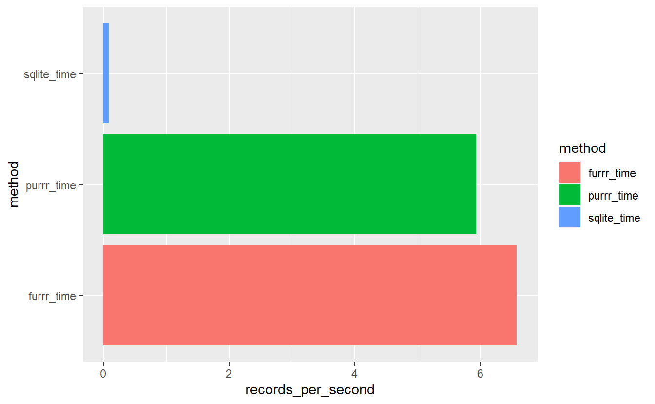
Even accounting for download times we can see that does not have much of an effect:
sql_v_purrr_v_furrr %>%
  mutate(download_time = download_time) %>%
  mutate(time_plus_download = if_else( method != 'sqlite_time',
                                       time + download_time,
                                       time)) %>%
  mutate(records_per_second = n_records/as.numeric(time_plus_download)) %>%
  ggplot(aes(x= method, y=records_per_second, fill=method)) +
  geom_bar(stat = "identity", position=position_dodge()) +
  coord_flip()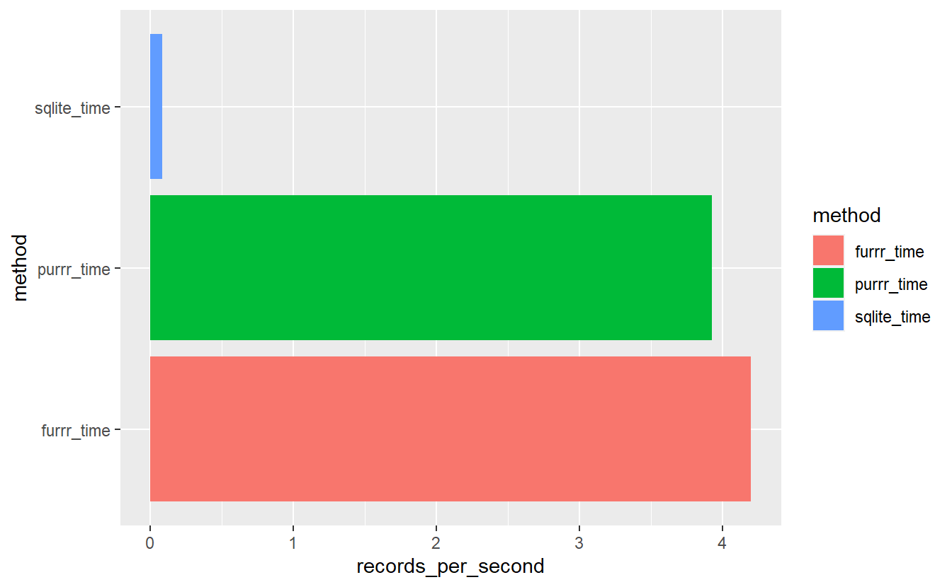
records_per_second_plus_download <- sql_v_purrr_v_furrr %>%
  mutate(download_time = download_time) %>%
  mutate(time_plus_download = if_else( method != 'sqlite_time',
                                       time + download_time,
                                       time)) %>%
  mutate(records_per_second = n_records/as.numeric(time_plus_download)) %>%
  select(method, records_per_second) %>%
  pivot_wider(names_from = method, values_from = records_per_second)

records_per_second_plus_download
#> # A tibble: 1 × 3
#>   sqlite_time purrr_time furrr_time
#>         <dbl>      <dbl>      <dbl>
#> 1      0.0824       3.93       4.20
Even accounting for download speeds locally with purrr our function is
records_per_second_plus_download$purrr_time / records_per_second_plus_download$sqlite_time
#> [1] 47.69075
times faster than with our SQLite connection and in this case furrr is
records_per_second_plus_download$furrr_time / records_per_second_plus_download$purrr_time
#> [1] 1.069567
times faster than purrr.
9.7 Compairing Outputs
The arsenal package contains a handy function comparedf to compare two data-frames. We can see that A_DATA_TBL_2.t_ks_result.purrr and A_DATA_TBL_2.t_ks_result.furrr match:
arsenal::comparedf(A_DATA_TBL_2.t_ks_result.purrr,
                   A_DATA_TBL_2.t_ks_result.furrr)
#> Compare Object
#>
#> Function Call:
#> arsenal::comparedf(x = A_DATA_TBL_2.t_ks_result.purrr, y = A_DATA_TBL_2.t_ks_result.furrr)
#>
#> Shared: 16 non-by variables and 67 observations.
#> Not shared: 0 variables and 0 observations.
#>
#> Differences found in 0/16 variables compared.
#> 0 variables compared have non-identical attributes.
However, A_DATA_TBL_2.t_ks_result.sql and A_DATA_TBL_2.t_ks_result.purrr do not:
arsenal::comparedf(A_DATA_TBL_2.t_ks_result.purrr,
                   A_DATA_TBL_2.t_ks_result.sql)
#> Compare Object
#>
#> Function Call:
#> arsenal::comparedf(x = A_DATA_TBL_2.t_ks_result.purrr, y = A_DATA_TBL_2.t_ks_result.sql)
#>
#> Shared: 16 non-by variables and 5 observations.
#> Not shared: 0 variables and 62 observations.
#>
#> Differences found in 0/16 variables compared.
#> 2 variables compared have non-identical attributes.
we can get a detailed summary of the outputs
compare.details <- arsenal::comparedf(A_DATA_TBL_2.t_ks_result.purrr,
                                      A_DATA_TBL_2.t_ks_result.sql) %>%
                           summary()
there are several tables to review
str(compare.details)
#> List of 9
#>  $ frame.summary.table     :'data.frame':    2 obs. of  4 variables:
#>   ..$ version: chr [1:2] "x" "y"
#>   ..$ arg    : chr [1:2] "A_DATA_TBL_2.t_ks_result.purrr" "A_DATA_TBL_2.t_ks_result.sql"
#>   ..$ ncol   : int [1:2] 16 16
#>   ..$ nrow   : int [1:2] 67 5
#>  $ comparison.summary.table:'data.frame':    13 obs. of  2 variables:
#>   ..$ statistic: chr [1:13] "Number of by-variables" "Number of non-by variables in common" "Number of variables compared" "Number of variables in x but not y" ...
#>   ..$ value    : num [1:13] 0 16 16 0 0 0 16 5 62 0 ...
#>  $ vars.ns.table           :'data.frame':    0 obs. of  4 variables:
#>   ..$ version : chr(0)
#>   ..$ variable: chr(0)
#>   ..$ position: int(0)
#>   ..$ class   : list()
#>  $ vars.nc.table           :'data.frame':    0 obs. of  6 variables:
#>   ..$ var.x  : chr(0)
#>   ..$ pos.x  : int(0)
#>   ..$ class.x: list()
#>   ..$ var.y  : chr(0)
#>   ..$ pos.y  : int(0)
#>   ..$ class.y: list()
#>  $ obs.table               :'data.frame':    62 obs. of  3 variables:
#>   ..$ version      : chr [1:62] "x" "x" "x" "x" ...
#>   ..$ ..row.names..: int [1:62] 6 7 8 9 10 11 12 13 14 15 ...
#>   ..$ observation  : int [1:62] 6 7 8 9 10 11 12 13 14 15 ...
#>  $ diffs.byvar.table       :'data.frame':    16 obs. of  4 variables:
#>   ..$ var.x: chr [1:16] "Feature" "mean_diff_est" "ttest.pvalue" "mean_Target" ...
#>   ..$ var.y: chr [1:16] "Feature" "mean_diff_est" "ttest.pvalue" "mean_Target" ...
#>   ..$ n    : num [1:16] 0 0 0 0 0 0 0 0 0 0 ...
#>   ..$ NAs  : num [1:16] 0 0 0 0 0 0 0 0 0 0 ...
#>  $ diffs.table             :'data.frame':    0 obs. of  7 variables:
#>   ..$ var.x        : chr(0)
#>   ..$ var.y        : chr(0)
#>   ..$ ..row.names..: chr(0)
#>   ..$ values.x     : list()
#>   .. ..- attr(*, "class")= chr "AsIs"
#>   ..$ values.y     : list()
#>   .. ..- attr(*, "class")= chr "AsIs"
#>   ..$ row.x        : int(0)
#>   ..$ row.y        : int(0)
#>  $ attrs.table             :'data.frame':    2 obs. of  3 variables:
#>   ..$ var.x: chr [1:2] "statistic" "parameter"
#>   ..$ var.y: chr [1:2] "statistic" "parameter"
#>   ..$ name : chr [1:2] "names" "names"
#>  $ control                 :List of 16
#>   ..$ tol.logical            :List of 1
#>   .. ..$ :function (x, y)
#>   ..$ tol.num                :List of 1
#>   .. ..$ :function (x, y, tol)
#>   ..$ tol.num.val            : num 1.49e-08
#>   ..$ int.as.num             : logi FALSE
#>   ..$ tol.char               :List of 1
#>   .. ..$ :function (x, y)
#>   ..$ tol.factor             :List of 1
#>   .. ..$ :function (x, y)
#>   ..$ factor.as.char         : logi FALSE
#>   ..$ tol.date               :List of 1
#>   .. ..$ :function (x, y, tol)
#>   ..$ tol.date.val           : num 0
#>   ..$ tol.other              :List of 1
#>   .. ..$ :function (x, y)
#>   ..$ tol.vars               : chr "none"
#>   ..$ max.print.vars         : logi NA
#>   ..$ max.print.obs          : logi NA
#>   ..$ max.print.diffs.per.var: num 10
#>   ..$ max.print.diffs        : num 50
#>   ..$ max.print.attrs        : logi NA
#>  - attr(*, "class")= chr "summary.comparedf"
this is the comparison.summary.table
compare.details$comparison.summary.table
#>                                                      statistic value
#> 1                                       Number of by-variables     0
#> 2                         Number of non-by variables in common    16
#> 3                                 Number of variables compared    16
#> 4                           Number of variables in x but not y     0
#> 5                           Number of variables in y but not x     0
#> 6        Number of variables compared with some values unequal     0
#> 7           Number of variables compared with all values equal    16
#> 8                             Number of observations in common     5
#> 9                        Number of observations in x but not y    62
#> 10                       Number of observations in y but not x     0
#> 11 Number of observations with some compared variables unequal     0
#> 12    Number of observations with all compared variables equal     5
#> 13                                    Number of values unequal     0
for instance compare.details$obs.table has the elements in A_DATA_TBL_2.t_ks_result.purrr (x) that are not within A_DATA_TBL_2.t_ks_result.sql (y):
compare.details$obs.table %>%
  head()
#>    version ..row.names.. observation
#> 6        x             6           6
#> 7        x             7           7
#> 8        x             8           8
#> 9        x             9           9
#> 10       x            10          10
#> 11       x            11          11
If we want the top 10 corresponding records we could do:
A_DATA_TBL_2.t_ks_result.purrr[compare.details$obs.table$observation[1:10],] %>%
  select(Feature, mean_diff_est , ttest.pvalue, kstest.pvalue) %>%
knitr::kable()| Feature | mean_diff_est | ttest.pvalue | kstest.pvalue |
|---|---|---|---|
| BPXDI1 | 2.0287700 | 0.0000000 | 0.0000000 |
| BPXDI3 | 1.4962007 | 0.0000000 | 0.0000000 |
| BPXDI2 | 1.9641076 | 0.0000000 | 0.0000000 |
| BPXSY4 | 16.4997779 | 0.0000000 | 0.0000000 |
| BPXCHR | -3.3841165 | 0.5185255 | 0.8169532 |
| BPXSY3 | 13.9986384 | 0.0000000 | 0.0000000 |
| Age | 31.4857235 | 0.0000000 | 0.0000000 |
| BPXSY2 | 14.4193913 | 0.0000000 | 0.0000000 |
| BPXSY1 | 14.8423483 | 0.0000000 | 0.0000000 |
| BPXDAR | 0.8349423 | 0.0689078 | 0.0164992 |
\(~\)
\(~\)