Chapter 17 Most Powerful Tests, Size of Union-Intersection and Intersection-Union Tests, p-Values(Lecture on 02/20/2020)

Example 17.1 (UMP Binomial Test) Let $X\sim Bin(2,\theta)$. We want to test $H_0:\theta=\frac{1}{2}$ versus $H_1:\theta=\frac{3}{4}$. Calculating the ratios of the p.m.f. gives $$\begin{equation} \frac{f(0|\theta=\frac{3}{4})}{f(0|\theta=\frac{1}{2})}=\frac{1}{4} \quad \frac{f(1|\theta=\frac{3}{4})}{f(1|\theta=\frac{1}{2})}=\frac{3}{4} \quad \frac{f(2|\theta=\frac{3}{4})}{f(2|\theta=\frac{1}{2})}=\frac{9}{4} \tag{17.1} \end{equation}$$ If we choose $\frac{3}{4}<k<\frac{9}{4}$, the Neyman-Perason Lemma says that the test that rejects $H_0$ if $X=2$ is the UMP level $\alpha=P(X=2|\theta=\frac{1}{2})=\frac{1}{4}$ test. If we choose $\frac{1}{4}<k<\frac{3}{4}$, the Neyman-Perason Lemma says that the test that rejects $H_0$ if $X=1$ or 2 is the UMP level $\alpha=P(X=1\,or\,2|\theta=\frac{1}{2})=\frac{3}{4}$ test. Choosing $k<\frac{1}{4}$ or $k>\frac{9}{4}$ yields the UMP level $\alpha=1$ or level $\alpha=0$ test.

Note that if $k=\frac{3}{4}$, then (16.11) says we must reject $H_0$ for the sample point $x=2$ and accept $H_0$ for $x=0$ but leaves our action for $x=1$ undetermined. If we accept $H_0$ for $x=1$, we get the UMP level $\alpha=\frac{1}{4}$ test as above. If we reject $H_0$ for $x=1$, we get the UMP level $\alpha=\frac{3}{4}$ test as above.

For a discrete distribution, the $\alpha$ level at which a test can be done is a function of the particular p.m.f. with which we are dealing. For continuous random variable, any $\alpha$ level is attainable.

Example 17.2 (UMP Normal Test) Let $X_1,\cdots,X_n$ be a random sample from a $N(\theta,\sigma^2)$ population, $\sigma^2$ known. The sample mean $\bar{X}$ is a sufficient statistic for $\theta$. Consider testing $H_0:\theta=\theta_0$ versus $H_1:\theta=\theta_1$ where $\theta_0>\theta_1$. The inequality (16.17), $g(\bar{x}|\theta_1)>kg(\bar{x}|\theta_0)$ is equivalent to $$\begin{equation} \bar{x}<\frac{(2\sigma^2\log k)/n-\theta_0^2+\theta_1^2}{2(\theta_1-\theta_0)} \tag{17.2} \end{equation}$$ The fact that $\theta_1-\theta_0<0$ was used to obatin this inequality. The right-hand side increases from $-\infty$ to $\infty$ as $k$ increases from 0 to $\infty$. Thus, by Corollary 16.1, the test with rejection region $\bar{x}<c$ is the UMP level $\alpha$ test, where $\alpha=P_{\theta_0}(\bar{X}<c)$. If a particular $\alpha$ is sepcified, then the UMP test rejects $H_0$ if $\bar{X}<c=-\frac{\sigma z_{\alpha}}{\sqrt{n}}+\theta_0$.

Definition 17.1 (Simple Hypotheses and Composite Hypotheses) Hypotheses that specify only one possible distribution for the sample $\mathbf{X}$ are called simple hypotheses, such as $H_0$ and $H_1$ in the Neyman-Pearson Lemma. If the hypotheses of intrest specify more than one possible distribution for the sample, then they are called composite hypotheses.

Definition 17.2 (One-sided Hypotheses and Two-sided Hypotheses) Hypotheses that assert that a univariate parameter is large, for example, $H:\theta\geq\theta_0$, or small, for example, $H:\theta<\theta_0$, are called one-sided hypotheses. Hypotheses that assert that a univariate parameter is either large or small, for example, $H:\theta\neq\theta_0$, are called two-sided hypotheses.

Definition 17.3 (Monotone Likelihood Ratio) A family of p.d.f. or p.m.f. $\{g(t|\theta):\theta\in\Theta\}$ for a univariate random variable $T$ with real-valued parameter $\theta$ has a monotone likelihood ratio (MLR) if, for every $\theta_2>\theta_1$, $\frac{g(t|\theta_2)}{g(t|\theta_1)}$ is a monotone (nonincreasing or nondecreasing) function of $t$ on $\{t:g(t|\theta_1)>0\,or\,g(t|\theta_2)>0\}$. Notice that $\frac{c}{0}$ is defined as $\infty$ if $0<c$.

Many common families of distributions have an MLR. For example, the normal (known variance, unknown mean), Poisson, and Binomial all have an MLR. Indeed, any regular exponential family with $g(t|\theta)=h(t)c(\theta)e^{\omega(\theta)t}$ has an MLR if $\omega(\theta)$ is a nondecreasing function.

Theorem 17.1 (Karlin-Rubin) Consider testing $H_0:\theta\leq\theta_0$ versus $H_1:\theta>\theta_0$. Suppose that $T$ is a sufficient statistic for $\theta$ and the family of p.d.f. or p.m.f. $\{g(t|\theta):\theta\in\Theta\}$ of $T$ has an MLR. Then for any $t_0$, the test that rejects $H_0$ if and only if $T>t_0$ is a UMP level $\alpha$ test, where $\alpha=P_{\theta_0}(T>t_0)$.

Proof. Let $\beta(\theta)=P_{\theta}(T>t_0)$ be the power function of the test. Fix $\theta^{\prime}>\theta_0$ and consider testing $H_0^{\prime}:\theta=\theta_0$ versus $H_1^{\prime}:\theta=\theta^{\prime}$. Since the family of p.d.f. or p.m.f. of $T$ has an MLR, $\beta(\theta)$ is nondecreasing, so

1. $\sup_{\theta\leq\theta_0}\beta(\theta)=\beta(\theta_0)=\alpha$, and this is a level $\alpha$ test.

2. If we define $k^{\prime}=\inf_{t\in\mathcal{T}}\frac{g(t|\theta^{\prime})}{g(t|\theta_0)}$, where $\mathcal{T}=\{t:t>t_0,\,either\,g(t|\theta^{\prime})>0\,or\,g(t|\theta_0)>0)\}$, it follows that $$\begin{equation} T>t_0 \Leftrightarrow \frac{g(t|\theta^{\prime})}{g(t|\theta_0)}>k^{\prime} \tag{17.3} \end{equation}$$ Together with Corollary 16.1, (i) and (ii) imply that $\beta(\theta^{\prime})\geq\beta^*(\theta^{\prime})$, where $\beta^*(\theta)$ is the power function for any other level $\alpha$ test of $H_0^{\prime}$, that is, any test satisfying $\beta(\theta_0)\leq\alpha$. However, any level $\alpha$ test of $H_0$ satisfies $\beta^*(\theta_0)\leq\sup_{\theta\in\Theta_0}\beta^*(\theta)\leq\alpha$. Thus, $\beta(\theta^{\prime})\geq\beta^*(\theta^{\prime})$ for any level $\alpha$ test of $H_0$. Thus, $\beta(\theta^{\prime})\geq \beta^*(\theta^{\prime})$ for any level $\alpha$ test of $H_0$. Since $\theta^{\prime}$ was arbitrary, the test is a UMP level $\alpha$ test.

By an analogous argument, it can be shown that under the conditions of Theorem 17.1, the test that rejects $H_0:\theta\geq\theta_0$ in favor of $H_1:\theta<\theta_0$ if and only if $T<t_0$ is a UMP level $\alpha=P_{\theta_0}(T<t_0)$ test.

Example 17.3 Consider testing $H_0^{\prime}:\theta\geq\theta_0$ versus $H_1^{\prime}:\theta<\theta_0$ using the test that rejects $H_0^{\prime}$ if $\bar{X}<-\frac{\sigma z_{\alpha}}{\sqrt{n}}+\theta_0$. As $\bar{X}$ is sufficient and its distribution has an MLR, it follows from Theorem 17.1 that the test is a UMP level $\alpha$ test in this problem.

As the power function of this test, $$\begin{equation} \beta(\theta)=P_{\theta}(\bar{X}<-\frac{\sigma z_{\alpha}}{\sqrt{n}}+\theta_0) \tag{17.4} \end{equation}$$ is a decreasing function of $\theta$ (since $\theta$ is a location parameter in the distribution of $\bar{X}$), the value of $\alpha$ is given by $\sup_{\theta\geq\theta_0}\beta(\theta)=\beta(\theta_0)=\alpha$.

Although most experimenters would choose to use a UMP level $\alpha$ test if they knew of one, unfortunately, for many problems there is no UMP level $\alpha$ test. That is, no UMP test exists because the class of level $\alpha$ tests is so large that no one test dominates all the others in terms of power. In such cases, a common method of continuing the search for a good test is to consider some subset of the class of level $\alpha$ tests and attempt to find a UMP test in this subset.

Example 17.4 (Nonexistence of UMP Test) Let $X_1,\cdots,X_n$ be i.i.d. $N(\theta,\sigma^2)$, $\sigma^2$ known. Consider testing $H_0:\theta=\theta_0$ versus $H_1:\theta\neq\theta_0$. For a specified value $\alpha$, a level $\alpha$ test in this problem is any test that satisfies $$\begin{equation} P_{\theta_0}(reject\,H_0)\leq \alpha \tag{17.5} \end{equation}$$ Consider an alternative parameter point $\theta_1<\theta_0$. Tha analysis in Example 17.3 shows that, among all tests that satisfy (17.5), the test that rejects $H_0$ if $\bar{X}<-\frac{\sigma z_{\alpha}}{\sqrt{n}}+\theta_0$ has the highest possible power at $\theta_1$. Call this Test 1. Furthermore, by necessity of the Neyman-Pearson Lemma, any other level $\alpha$ test that has as high a power as Test 1 at $\theta_1$ must have the same rejection region as Test 1 except possibly for a set $A$ satisfying $\int_{A}f(\mathbf{x}|\theta_i)d\mathbf{x}=0$. Thus, if a UMP level $\alpha$ test exists for this problem, it must be Test 1 because no other test has as high a power as Test 1 at $\theta_1$.

Now consider Test 2, which rejects $H_0$ if $\bar{X}>\frac{\sigma z_{\alpha}}{\sqrt{n}}+\theta_0$. Test 2 is also a level $\alpha$ test. Let $\beta_i(\theta)$ denote the power function of Test $i$, for any $\theta_2>\theta_0$, $$\begin{equation} \begin{split} \beta_2(\theta_2)&=P_{\theta_2}(\bar{X}>\frac{\sigma z_{\alpha}}{\sqrt{n}}+\theta_0)\\ &=P_{\theta_2}(\frac{\bar{X}-\theta_2}{\sigma/\sqrt{n}}> z_{\alpha}+\frac{\theta_0-\theta_2}{\sigma/\sqrt{n}})\\ &>P(Z>z_{\alpha})=P(Z<-z_{alpha})\\ &>P_{\theta_2}(\frac{\bar{X}-\theta_2}{\sigma/\sqrt{n}}< -z_{\alpha}+\frac{\theta_0-\theta_2}{\sigma/\sqrt{n}})\\ &=P_{\theta_2}(\bar{X}<-\frac{\sigma z_{\alpha}}{\sqrt{n}}+\theta_0)\\ &=\beta_1(\theta_2) \end{split} \tag{17.6} \end{equation}$$

Thus, Test 1 is not a UMP level $\alpha$ test because Test 2 has a higher power than Test 1 at $\theta_2$. Earlier we showed that if there were a UMP level $\alpha$ test, it would have to be Test 1. Therefore, no UMP level $\alpha$ test exists in this problem.

The sufficiency part of the Neyman-Pearson Lemma is used to construct UMP level $\alpha$ tests. The necessity part of the lemma is used to show the nonexistence of a UMP level $\alpha$ test.

Example 17.5 (Unbiased Test) When no UMP level $\alpha$ test exists within the class of all tests, we might try to find a UMP level $\alpha$ test within the class of unbiased tests. The power function $\beta_3(\theta)$ of Test 3, whihc rejects $H_0:\theta=\theta_0$ in favor of $H_1:\theta\neq\theta_0$ if and only if $\bar{X}>\frac{\sigma z_{\alpha/2}}{\sqrt{n}}+\theta_0$ or $\bar{X}<-\frac{\sigma z_{\alpha/2}}{\sqrt{n}}+\theta_0$ as well as $\beta_1(\theta)$ and $\beta_2(\theta)$ in Example 17.4 is shown in Figure 17.1. Test 3 is actually a UMP unbiased level $\alpha$ test.

Note that although Test 1 and Test 2 have slightly higher powers than Test 3 for some parameter points, Test 3 has much higher power than Test 1 and Test 2 at other parameter points. For example, $\beta_3(\theta_2)$ is near 1, whereas $\beta_1(\theta_2)$ is near O. If the interest is in rejecting $H_0$ for both large and small values of 0, Figure 17.1 shows that Test 3 is better overall than either Test 1 or Test 2.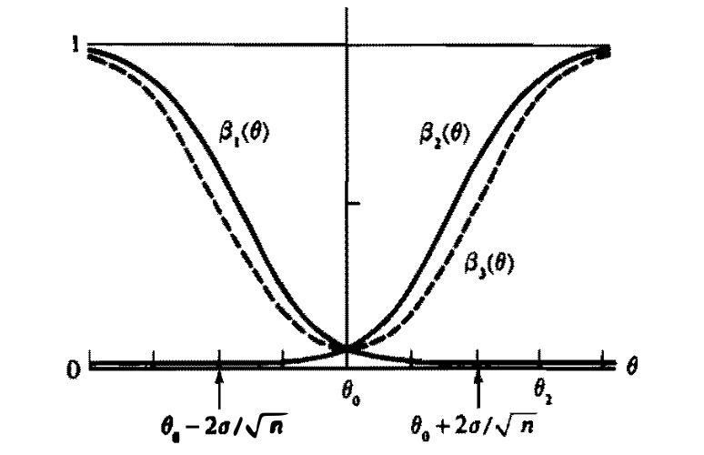

FIGURE 17.1: Power functions for three tests

Because of the simple way in which they are constructed, the sizes of union-intersection tests (UIT) and intersection union tests (IUT) can often be bounded above by the sizes of some other tests. Such bounds are useful if a level $\alpha$ test is wanted, but the size of the UIT or IUT is too difficult to evaluate.

Let $\lambda_{\gamma}(\mathbf{x})$ be the LRT statistic for testing $H_{0_{\gamma}}:\theta\in\Theta_{\gamma}$ versus $H_{1_{\gamma}}:\theta\in\Theta_{\gamma}^c$, and let $\lambda(\mathbf{x})$ be the LRT statistic for testing $H_0:\theta\in\Theta_0$ versus $H_1:\theta\in\Theta_0^c$.

Theorem 17.2 Consider testing $H_0:\theta\in\Theta_0$ versus $H_1:\theta\in\Theta_0^c$, where $\theta_0=\bigcap_{\gamma\in\Gamma}\Theta_{\gamma}$ and $\lambda_{\gamma}(\mathbf{x})$ is defined as previous. Define $T(\mathbf{x})=\inf_{\gamma\in\Gamma}\lambda_{\gamma}(\mathbf{x})$, and form the UIT with rejection region $\{\mathbf{x}:\lambda_{\gamma}(\mathbf{x})<c,\gamma\in\Gamma\}=\{\mathbf{x}:T(\mathbf{x})<c\}$. Also consider the usual LRT with rejection region $\{\mathbf{x}:\lambda(\mathbf{x})<c\}$. Then

1. $T(\mathbf{x})\geq \lambda(\mathbf{x})$ for every $\mathbf{x}$;

2. If $\beta_T(\theta)$ and $\beta_{\lambda}(\theta)$ are the power functions for the tests based on $T$ and $\lambda$, respectively, then $\beta_T(\theta)\leq\beta_{\lambda}(\theta)$ for every $\theta\in\Theta$;

3. If the LRT is a level $\alpha$ test, then the UIT is a level $\alpha$ test.

Proof. Since $\Theta_0=\bigcap_{\gamma\in\Gamma}\Theta_{\gamma}\subset\Theta_{\gamma}$ for any $\gamma$, from Definition 15.4 we see that for any $\mathbf{x}$, $$\begin{equation} \lambda_{\gamma}(\mathbf{x})\geq \lambda(\mathbf{x}),\forall\gamma\in\Gamma \tag{17.7} \end{equation}$$ because the region of maximization is bigger for the individual $\lambda_{\gamma}$. Thus, $T(\mathbf{x})=\inf_{\gamma\in\Gamma}\lambda_{\gamma}(\mathbf{x})\geq\lambda(\mathbf{x})$, proving (a). By (a), $\{\mathbf{x}:T(\mathbf{x})<c\}\subset\{\mathbf{x}:\lambda(\mathbf{x})<c\}$, so $$\begin{equation} \beta_T(\theta)=P_{\theta}(T(\mathbf{X})<c)\leq P_{\theta}(\lambda(\mathbf{X})<c)=\beta_{\lambda}(\theta) \tag{17.8} \end{equation}$$ proving (b). Since (b) holds for every $\theta$, $\sup_{\theta\in\Theta_0}\beta_T(\theta)\leq\sup_{\theta\in\Theta_0}\beta_{\lambda}(\theta)\leq\alpha$, proving (c).

Example 17.6 (An equivalence) In some situations, $T(\mathbf{x})=\lambda(\mathbf{x})$ in Theorem 17.2. The UIT built up from indicidual LRTs is the same as the overall LRT. This was the case in Example 15.6. There the UIT formed from two one-sided t tests was equivalent to the two-sided LRT.

Theorem 17.2 says the LRT is uniformly more powerful than the UIT. Why should we consider UIT?

• UIT has a smaller Type I Error probability for every $\theta\in\Theta_0$.

• If $H_0$ is rejected, we may wish to look at the individual tests of $H_{0_{\gamma}}$ to see why.

Theorem 17.3 Let $\alpha_{\gamma}$ be the size of the test of $H_{0_{\gamma}}$ with rejection region $R_{\gamma}$. Then the IUT with rejection region $R=\bigcap_{\gamma\in\Gamma}R_{\gamma}$ is a level $\alpha=\sup_{\gamma\in\Gamma}\alpha_{\gamma}$ test.

Proof. Let $\theta\in\Theta_0$. Then $\theta\in\Theta_{\gamma}$ for some $\gamma$ and $$\begin{equation} P_{\theta}(\mathbf{X}\in R)\leq P_{\theta}(\mathbf{X}\in R_{\gamma})\leq\alpha_{\gamma}\leq\alpha \tag{17.9} \end{equation}$$ Since $\theta\in\Theta_0$ was arbitrary, the IUT is a level $\alpha$ test.

• Typically the individual rejection regions $R_{\gamma}$ are choosen so that $\alpha_{\gamma}=\alpha$ for all $\gamma$. In such case, the resulting IUT is a level $\alpha$ test.

• Theorem 17.2 applies only to UITs constructed from likelihood ratio tests. Theorem 17.3 applies to any IUT.

• The bound in Theorem 17.2 is the size of the LRT, which may be difficult to compute. In Theorem 17.3, any test of $H_{0_{\gamma}}$ with known size $\alpha_{\gamma}$ can be used and then then the upper bound on the size of the IUT is given in terms of the known sizes $\alpha_{\gamma},\gamma\in\Gamma$.

Theorem 17.4 Consider testing $H_0:\theta\in\bigcup_{j=1}^k\Theta_j$, where $k$ is a finite positive integer. For each $j=1,\cdots,k$, let $R_j$ be the rejection region of a level $\alpha$ test of $H_{0_j}$. Suppose that for some $i=1,\cdots,k$, there exists a sequence of parameter points, $\theta_l\in\Theta_i$, $l=1,2,\cdots$, such that

1. $\lim_{l\to\infty}P_{\theta_l}(\mathbf{X}\in R_i)=\alpha$,

2. for each $j=1,\cdots,k$, $j\neq i$, $\lim_{l\to\infty}P_{\theta_l}(\mathbf{X}\in R_j)=1$.

Then, the IUT with rejection region $R=\bigcap_{j=1}^kR_j$ is a size $\alpha$ test.

Proof. By Theorem 17.3, $R$ is a level $\alpha$ test, that is $$\begin{equation} \sup_{\theta\in\Theta_0}P_{\theta}(\mathbf{X}\in R)\leq\alpha \tag{17.10} \end{equation}$$

But, because all the parameter points $\theta_l$ satisfy $\theta_l\in\Theta_i\subset\Theta_0$, $$\begin{equation} \begin{split} \sup_{\theta\in\Theta_0}P_{\theta}(\mathbf{X}\in R)&\geq \lim_{l\to\infty}P_{\theta_l}(\mathbf{X}\in R)\\ =\lim_{l\to\infty}P_{\theta_l}(\mathbf{X}\in\bigcap_{j=1}^kR_j)\\ &\geq \lim_{l\to\infty}]\sum_{j=1}^kP_{\theta_l}(\mathbf{X}\in R_j)-(k-1) \quad (Bonferroni\, Inequality)\\ &=(k-1)+\alpha-(k-1)=\alpha \end{split} \tag{17.11} \end{equation}$$

This and (17.10) imply the test has size exactly equal to $\alpha$.

In IUTs, only the marginal distribution of each test is needed to be considered, which eliminate the difficulty of considering the joint distribution, which may need to work with correlations.

Definition 17.4 (p-Values) A p-value $P(\mathbf{X})$ is a test statistic satisfying $0\leq p(\mathbf{x})\leq 1$ for every sample point $\mathbf{x}$. Small values of $p(\mathbf{X})$ give evidence that $H_1$ is true. A p-value is valid if, for every $\theta\in\Theta_0$ and every $0\leq\alpha\leq 1$, $$\begin{equation} P_{\theta}(p(\mathbf{X})\leq\alpha)\leq\alpha \tag{17.12} \end{equation}$$

• If $p(\mathbf{X})$ is a valid p-value, it is easy to construct a level $\alpha$ test based on $p(\mathbf{X})$. The test that rejects $H_0$ if and only if $p(\mathbf{X})\leq \alpha$ is a level $\alpha$ test because of (17.12).

• An advantage to reporting a test result via a p-value is that each reader can choose the $\alpha$ he or she considers appropriate and then can compare the reported p(x) to $\alpha$ and know whether these data lead to acceptance or rejection of $H_0$.

• The smaller the p-value, the stronger the evidence for rejecting $H_0$. Hence, a p-value reports the results of a test on a more continuous scale, rather than just the dichotomous decision “Accept $H_0$” or “Reject $H_0$”.

Theorem 17.5 Let $W(\mathbf{X})$ be a test statistic such that large values of W gives evidence that $H_1$ is true. For each sample point $\mathbf{x}$, define $$\begin{equation} p(\mathbf{x})=\sup_{\theta\in\Theta_0}P_{\theta}(W(\mathbf{X})\geq W(\mathbf{x})) \tag{17.13} \end{equation}$$ Then $p(\mathbf{X})$ is a valid p-value.

Proof. Fix $\theta\in\Theta_0$. Let $F_{\theta}(\omega)$ denote the c.d.f. of $-W(\mathbf{X})$. Define $$\begin{equation} p_{\theta}(\mathbf{x})=P_{\theta}(W(\mathbf{X})\geq W(\mathbf{x}))=P_{\theta}(-W(\mathbf{X})\leq-W(\mathbf{x}))=F_{\theta}(-W(\mathbf{x})) \tag{17.14} \end{equation}$$ Then the random variable $P_{\theta}(\mathbf{X})$ us equal to $F_{\theta}(-W(\mathbf{X}))$. by probability integral transformation, for every $0\leq\alpha\leq 1$, $P_{\theta}(p_{\theta}(\mathbf{X})\leq\alpha)\leq\alpha$. Because $p(\mathbf{x})=\sup_{\theta^{\prime}\in\Theta_0}p_{\theta^{\prime}}(\mathbf{x})\geq p_{\theta}(\mathbf{x})$ for every $\mathbf{x}$, $$\begin{equation} P_{\theta}(p(\mathbf{X})\leq\alpha)\leq P_{\theta}(p_{\theta}(\mathbf{X})\leq\alpha)\leq\alpha \tag{17.15} \end{equation}$$ This is true for every $\theta\in\Theta_0$ and for every $0\leq\alpha\leq 1$; $p(\mathbf{X})$ is a valid p-value.

Example 17.7 (Two-sided Normal p-Value) Let $X_1,\cdots,X_n$ be a random sample from $N(\mu,\sigma^2)$ population. Consider testing $H_0:\mu=\mu_0$ versus $H_1:\mu\neq\mu_0$. The LRT rejects $H_0$ for large values of $W(\mathbf{X})=\frac{|\bar{X}-\mu_0|}{S/\sqrt{n}}$. If $\mu=\mu_0$, regardless of the value of $\sigma$, $\frac{\bar{X}-\mu_0}{S/\sqrt{n}}$ has a t-distribution with $n-1$ degrees of freedom. Thus, in calculating (17.13), the probability is the same for all values of $\theta$, that is, all values of $\sigma$. Thus, the p-value from (17.13) for this two-sided t test is $p(\mathbf{x})=2P(T_{n-1}\geq \frac{\bar{x}-\mu_0}{s/\sqrt{n}})$, where $T_{n-1}$ has a t-distribution with $n-1$ degrees of freedom.

Example 17.8 (One-sided Normal p-Value) Let $X_1,\cdots,X_n$ be a random sample from $N(\mu,\sigma^2)$ population. Consider testing $H_0:\mu\leq\mu_0$ versus $H_1:\mu>\mu_0$. The LRT rejects $H_0$ for large values of $W(\mathbf{X})=\frac{\bar{X}-\mu_0}{S/\sqrt{n}}$. Consider any $\mu\leq\mu_0$ and any $\sigma$, $$\begin{equation} \begin{split} P_{\mu,\sigma}(W(\mathbf{X})\geq W(\mathbf{x}))&=P_{\mu,\sigma}(\frac{\bar{X}-\mu_0}{S/\sqrt{n}}\geq W(\mathbf{x}))\\ &=P_{\mu,\sigma}(\frac{\bar{X}-\mu}{S/\sqrt{n}}\geq W(\mathbf{x})+\frac{\mu_0-\mu}{S/\sqrt{n}})\\ &=P_{\mu,\sigma}(T_{n-1}\geq W(\mathbf{x})+\frac{\mu_0-\mu}{S/\sqrt{n}})\\ \leq P(T_{n-1}\geq W(\mathbf{x})) \end{split} \tag{17.16} \end{equation}$$
The inequality in the last line is true becasue $\mu_0\geq\mu$ and $\frac{\mu_0-\mu}{S/\sqrt{n}}$ is a nonnegative random variable. The subscript on $P$ is dropped because the probability does not depend on $(\mu,\sigma)$. Furthermore, $$\begin{equation} P(T_{n-1}\geq W(\mathbf{x}))=P_{\mu_0,\sigma}(\frac{\bar{X}-\mu_0}{S/\sqrt{n}}\geq W(\mathbf{x}))=P_{\mu_0,\sigma}(W(\mathbf{X})\geq W(\mathbf{x})) \tag{17.17} \end{equation}$$ beacuse $\frac{\bar{X}-\mu_0}{S/\sqrt{n}}\sim T_{n-1}$ given $\theta=\theta_0$ and this probability is one of those considered in the calculation of the supremum in (17.13) because $(\mu_0,\sigma)\in\Theta_0$. Thus, the p-value from (17.13) for this one-sided t test is $p(\mathbf{x})=P(T_{n-1}\geq W(\mathbf{x}))=P(T_{n-1}\geq \frac{\bar{x}-\mu_0}{s/\sqrt{n}})$.

Corollary 17.1 (p-Value Conditioning on Sufficient Statistic) Another method for definition a valid p-value involves conditioning on a sufficient statistic. Suppose $S(\mathbf{X})$ is a sufficient statisitc for the model $\{f(\mathbf{x}|\theta):\theta\in\Theta_0\}$. If the null hypothesis is true, the conditional distribution of $\mathbf{X}$ given $S=s$ does not depend on $\theta$. Again, let $W(\mathbf{X})$ denote a test statistic for which large values give evidence that $H_1$ is true. Then, for each sample point $\mathbf{x}$ define $$\begin{equation} p(\mathbf{x})=P(W(\mathbf{X})\geq W(\mathbf{x})|S=S(\mathbf{x})) \tag{17.18} \end{equation}$$ Considering only the single distribution that is the conditional distribution of $\mathbf{X}$ given $S=s$, we see that, for any $0\leq\alpha\leq 1$, $P(p(\mathbf{X})\leq\alpha|S=s)\leq\alpha$. Then, for any $\theta\in\Theta_0$, unconditionally we have $$\begin{equation} P_{\theta}(p(\mathbf{X})\leq\alpha)=\sum_{s}P(p(\mathbf{X})\leq\alpha|S=s)P_{\theta}(S=s)\leq\sum_{s}\alpha P_{\theta}(S=s)\leq\alpha \tag{17.19} \end{equation}$$

Thus, $p(\mathbf{X})$ defined by (17.18) is a valid p-value.

The sum can be replaced by integrals for continuous $S$, but this method is usually used for discrete $S$.

Example 17.9 (Fisher Exact Test) Let $S_1$ and $S_2$ be independent observations with $S_1\sim Bin(n_1,p_1)$ and $S_2\sim Bin(n_2,p_2)$. Consider testing $H_0:p_1=p_2$ versus $H_1:p_1>p_2$. Under $H_0$, if we let $p$ denote the common value of $p_1=p_2$, the joint p.m.f. of $(S_1,S_2)$ is

$$\begin{equation} \begin{split} f(s_1,s_2|p)&={{n_1} \choose {s_1}}p^{s_1}(1-p)^{n_1-s_1}{{n_2} \choose {s_2}}p^{s_2}(1-p)^{n_2-s_2}\\ &={{n_1} \choose {s_1}}{{n_2} \choose {s_2}}p^{s_1+s_2}(1-p)^{n_1+n_2-(s_1+s_2)} \end{split} \tag{17.20} \end{equation}$$

Thus, $S=S_1+S_2$ is a sufficient statistic under $H_0$. Given the value of $S=s$, it is reasonable to use $S_1$ as a test statistic and reject $H_0$ in favor of $H_1$ for large values of $S_1$, because large values of $S_1$ correspond to small values of $S_2=s-S_1$. The conditional distribution of $S_1$ given $S=s$ is $HyperGeo(n_1+n_2,n_1,s)$. Thus, the conditional p-value in (17.18) is $$\begin{equation} p(s_1,s_2)=\sum_{j=s_1}^{\min\{n_1,s\}}f(j|s) \tag{17.21} \end{equation}$$ the sum of hypergeometric probabilities. The test defined by this p-value is called Fisher Exact Test.