Chapter 16 Error Probabilities, Power Function, Most Powerful Tests(Lecture on 02/18/2020)

Usually, hypothesis tests are evaluated and compared through their probabilities of making mistakes.

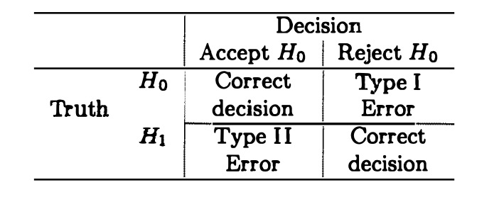
Definition 16.1 (Type of Errors) A hypothesis test of $H_0:\theta\in\Theta_0$ versus $H_1:\theta\in\Theta_0^c$ might make one of two types of errors, Type I Error and Type II Error. If $\theta\in\Theta_0$ but the hypothesis test incorrectly decides to reject $H_0$, then the test has made a Type I Error. If $\theta\in\Theta_0^c$ but the test decides to accept $H_0$, a $Type II Error$ has been made. Figure 16.1 illustrate this.

$\label{fig:16001}Two types of errors in hypothesis testing$

FIGURE 16.1: Two types of errors in hypothesis testing

Suppose $R$ denotes the rejection region for a test. Then for $\theta\in\Theta_0$, the test will make a mistake if $\mathbf{x}\in R$, so the porbability of a Type I Error is $P_{\theta}(\mathbf{X}\in R)$. For $\theta\in\Theta_0^c$, the probability of a Type II Error is $P_{\theta}(\mathbf{X}\in R^c)=1-P_{\theta}(\mathbf{X}\in R)$. The function of $\theta$, $P_{\theta}(\mathbf{X}\in R)$ contains all the information about the test with rejection region $R$.

Definition 16.2 (Power Function) The power function of a hypothesis test with rejection region $R$ is the function of $\theta$ defined by $\beta(\theta)=P_{\theta}(\mathbf{X}\in R)$.

The ideal power function is 0 for all $\theta\in\Theta_0$ and 1 for all $\theta\in\Theta_0^c$. Except in trivial situations, this ideal cannot be attained. A good test have power function near 1 for mose $\theta\in\Theta_0^c$ and near 0 for most $\theta\in\Theta_0$.

Example 16.1 (Binomial Power Function) Let $X\sim Bin(5,\theta)$. Consider testing $H_0:\theta\leq\frac{1}{2}$ versus $H_1:\theta>\frac{1}{2}$. Consider first the test that rejects $H_0$ if and only if all “successes” are observed. The power function for this test is \[\begin{equation} \beta_1(\theta)=P_{\theta}(\mathbf{X}\in R)=P_{\theta}(\mathbf{X}=5)=\theta^5 \tag{16.1} \end{equation}\]

In examing this power function, we might decide that although the probability of Type I Error is acceptable low ($\beta_1(\theta)\leq(\frac{1}{2})^5=0.0312$) for all $\theta\leq\frac{1}{2}$, the probability of a Type II Error is too high ($\beta_1(\theta)$ is too small) for most $\theta>\frac{1}{2}$. The probability of a Type II Error is less than $\frac{1}{2}$ only if $\theta>(\frac{1}{2})^{1/5}=0.87$. To achiece samller Type II Error probabilities, we might consider using the test that rejects $H_0$ if $X=3,4,5$. The power function is then \[\begin{equation} \beta_1(\theta)={5 \choose 3}\theta^3(1-\theta)^2+{5 \choose 4}\theta^4(1-\theta)+\theta^5 \tag{16.2} \end{equation}\] The second test has achieved a smaller Type II error probability in that $\beta_2(\theta)$ is larger for $\theta>\frac{1}{2}$. But the Type I Error probability is larger for the second test as $\beta_2(\theta)$ is larger for $\theta\leq\frac{1}{2}$. If a choice is to be made between these two tests, the researcher must decide which error structure, that described by $\beta_1(\theta)$ or that described by $\beta_2(\theta)$ is more acceptable. The two power function is shown in Figure 16.2.

$\label{fig:16002}Power functions for Binomial distribution example$

FIGURE 16.2: Power functions for Binomial distribution example

Example 16.2 (Normal Power Function) Let $X_1,\cdots,X_n$ be a random sample from a $N(\theta,\sigma^2)$ population, $\sigma^2$ known. An LRT of $H_0:\theta\leq\theta_0$ is a test that rejects $H_0$ if $\frac{\bar{X}-\theta_0}{\sigma/\sqrt{n}}>c$. The constant $c$ can be any positive number. The power function of this test is \[\begin{equation} \begin{split} \beta(\theta)&=P_{\theta}(\frac{\bar{X}-\theta_0}{\sigma/\sqrt{n}}>c)\\ &=P_{\theta}(\frac{\bar{X}-\theta}{\sigma/\sqrt{n}}>c+\frac{\theta_0-\theta}{\sigma/\sqrt{n}})\\ &=P(Z>c+\frac{\theta_0-\theta}{\sigma/\sqrt{n}}) \end{split} \tag{16.3} \end{equation}\] where $Z$ is a standard normal random variable. As $\theta$ increases from $-\infty$ to $\infty$, this normal probability increases from 0 to 1. Therefore, $\beta(\theta)$ is an increasing function of $\theta$, with $\lim_{\theta\to-\infty}\beta(\theta)=0$, $\lim_{\theta\to\infty}\beta(\theta)=1$ and $\beta(\theta_0)=\alpha$ if $P(Z>c)=\alpha$. The shape of this power function is shown in Figure 16.3.

$\label{fig:16003}Shape of power function for normal distribution.$

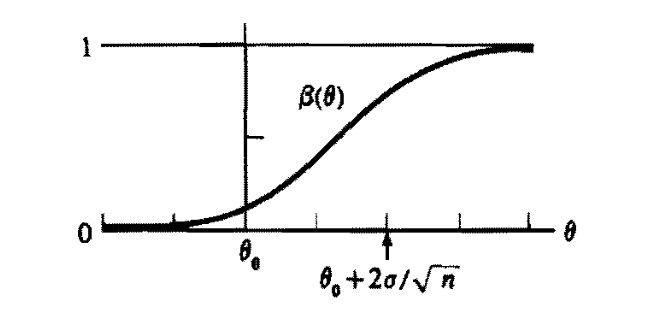
FIGURE 16.3: Shape of power function for normal distribution.

Typically, the power function of a test will depend on the sample size $n$. If $n$ can be chosen by the experimenter, consideration of the power function might help determine what sample size is appropriate in an experiment.

Example 16.3 Suppose the experimenter wishes to have a maximum Type I Error probability of 0.1. Suppose, in addition, the experimenter wishes to have a maximum Type II Error of probability of 0.2 if $\theta\geq\theta_0+\sigma$. We now show how to choose $c$ and $n$ to achieve these goals, using a test that rejects $H_0:\theta\leq\theta_0$ if $\frac{\bar{X}-\theta_0}{\sigma/\sqrt{n}}>c$. The power function of such a test is \[\begin{equation} \beta(\theta)=P(Z>c+\frac{\theta_0-\theta}{\sigma/\sqrt{n}}) \tag{16.4} \end{equation}\] Becasue $\beta(\theta)$ is increasing in $\theta$, the requirements will be met if $\beta(\theta_0)=0.1$ and $\beta(\theta_0+\sigma)=0.8$. By choosing $c=1.28$, we achieve $\beta(\theta_0)=P(Z>1.28)=0.1$, regradless of $n$. Now we wish to choose $n$ so that $\beta(\theta_0+\sigma)=P(Z>1.28-\sqrt{n})=0.8$. But $P(Z>-0.84)=0.8$ so setting $1.28-\sqrt{n}=-0.84$ and solving for $n$ yield $n=4.49$. Round up we have $n=5$.

For a fixed sample size, it is usually impossible to make both types of error probabilities arbitrarily small. In searching for a good test, it is common to restrict consideration to tests that control the Type I Error probability at a specified level. Within this class of tests we then search for tests that have Type II Error probability that is as small as possible.

Definition 16.3 (Size $\alpha$ Test) For $0\leq\alpha\leq 1$, a test with power function $\beta(\theta)$ is a size $\alpha$ test if $\sup_{\theta\in\Theta_0}\beta(\theta)=\alpha$.

Definition 16.4 (Level $\alpha$ Test) For $0\leq\alpha\leq 1$, a test with power function $\beta(\theta)$ is a level $\alpha$ test if $\sup_{\theta\in\Theta_0}\beta(\theta)\leq\alpha$.

The set of level $\alpha$ tests contains the set of size $\alpha$ tests. A size $\alpha$ test is usually more computationally hard to construct than a level $\alpha$ tests.
Experimenters commonly specify the level of the test they wish to use, tyoical choices being $\alpha=0.01,0.05,0.10$. In fixing the level of the test, the experimenter is controlling only the Type I Error probabilities, not the Type II Error. If this approach is taken, the experimenter should specify the null and alternative hypotheses so that it is most important to control the Type I Error probability.

Definition 16.5 (Research Hypothesis) Suppose an experimenter expects an experiment to give support to a particular hypothesis, but she does not wish to make the assertion unless the data really do give convincing support. The test can be set up so that the alternative hypothesis is the one that she expects the data to support, and hopes to prove. In this case, the alternative hypothesis is called research hypothesis. By using a level $\alpha$ test with small $\alpha$, the experimenter is guarding against saying the data support the research hypothesis when it actually not.

The restriction to size $\alpha$ tests lead to the choice of one out of the class of tests.

Example 16.4 (Size of LRT) In general, a size $\alpha$ LRT is constructed by choosing $c$ such that $\sup_{\theta\in\Theta_0}P_{\theta}(\lambda(\mathbf{X})\leq c)=\alpha$. In Example 15.1, $\Theta_0$ consists of the single point $\theta=\theta_0$ and $\sqrt{n}(\bar{X}-\theta_0)\sim N(0,1)$ if $\theta=\theta_0$. So the test reject $H_0$ if $|\bar{X}-\theta_0|\geq\frac{z_{\alpha/2}}{\sqrt{n}}$ where $z_{\alpha/2}$ satisfies $P(Z\geq z_{\alpha/2})=\alpha/2$ with $Z\sim N(0,1)$, is the size $\alpha$ LRT. Specifically, this corresponds to choosing $c=exp(-z^2_{\alpha/2}/2)$ but it is not necessary to calculate it out.

For the problem in Example 15.2, finding a size $\alpha$ LRT is done as follows. The LRT rejects $H_0$ if $\min_iX_i\geq c$, where $c$ is chosen so that this is a size $\alpha$ test. If $c=-\frac{\log\alpha}{n}+\theta_0$, then \[\begin{equation} P_{\theta_0}(\min_iX_i\geq c)=e^{-n(c-\theta_0)}=\alpha \tag{16.5} \end{equation}\] Since $\theta$ is a location parameter of $\min_iX_i$, \[\begin{equation} P_{\theta}(\min_iX_i\geq c)\leq P_{\theta_0}(\min_iX_i\geq c),\quad \forall\theta\leq\theta_0 \tag{16.6} \end{equation}\] Thus \[\begin{equation} \sup_{\theta\in\Theta_0}\beta(\theta)=\sup_{\theta\leq\theta_0}P_{\theta}(\min_iX_i\geq c)=P_{\theta_0}(\min_iX_i\geq c)=\alpha \tag{16.7} \end{equation}\] and this $c$ yields the size $\alpha$ LRT.

Definition 16.6 (Cutoff Points) We use a series of notations to represent the probability of having probability to the right of it for the corresponding distributions. Such as

$z_{\alpha}$ satisfies $P(Z>z_{\alpha})=\alpha$ where $Z\sim N(0,1)$.
$t_{n-1,\alpha/2}$ satisfies $P(T_{n-1}>t_{n-1,\alpha/2})=\alpha/2$ where $T_{n-1}\sim t_{n-1}$.
$\chi^2_{p,1-\alpha}$ satisfies $P(\chi_p^2>\chi^2_{p,1-\alpha})=1-\alpha$ where $\chi_p^2\sim \chi_p^2$.

$z_{\alpha}, t_{n-1,\alpha/2}$ and $\chi^2_{p,1-\alpha}$ are known as cutoff points.

Example 16.5 (Size of Union-Intersection Test) The problem of finding a size $\alpha$ union-intersection test in Example 15.6 involves finding constants $t_L$ and $t_U$ such that \[\begin{equation} \sup_{\theta\in\Theta_0}P_{\theta}(\frac{\bar{X}-\mu_0}{\sqrt{S^2/n}}\geq t_L\,or\,\frac{\bar{X}-\mu_0}{\sqrt{S^2/n}}\leq t_U)=\alpha \tag{16.8} \end{equation}\] But for any $(\mu,\sigma^2)=\boldsymbol\theta\in\Theta_0$, $\mu=\mu_0$ and thus $\frac{\bar{X}-\mu_0}{\sqrt{S^2/n}}$ has a t-distribution with n-1 degrees of freedom. So any choice of $t_U=t_{n-1,1-\alpha_1}$ and $t_L=t_{n-1,\alpha_2}$ with $\alpha_1+\alpha_2=\alpha$ will yield a test with Type I Error probability of exactly $\alpha$. The ususal choice is $t_L=-t_U=t_{n-1,\alpha/2}$.

Definition 16.7 (Unbiased Test) A test with power function $\beta(\theta)$ is unbiased if $\beta(\theta^{\prime})\geq\beta(\theta^{\prime\prime})$ for every $\theta^{\prime}\in\Theta_0^c$ and $\theta^{\prime\prime}\in\Theta_0$.

Example 16.6 Assume the setting in Example 16.2, an LRT of $H_0:\theta\leq\theta_0$ versus $H_1:\theta>\theta_0$ has power function \[\begin{equation} \beta(\theta)=P(Z>c+\frac{\theta_0-\theta}{\sigma/\sqrt{n}}) \tag{16.9} \end{equation}\] where $Z\sim N(0,1)$. Since $\beta(\theta)$ is an increasing function of $\theta$ for fixed $\theta_0$, it follows that \[\begin{equation} \beta(\theta)>\beta(\theta_0)=\max_{t\leq\theta_0}\beta(t),\quad\forall\theta>\theta_0 \tag{16.10} \end{equation}\] and hence, that the test is unbiased.

There are usually more than one size $\alpha$ tests, likelihood ratio tests, unbiased tests, etc. We can imposed some restrictions to narrow consideration to one specific test.

Definition 16.8 (Uniformly Most Powerful Class $\mathcal{C}$ Test) Let $\mathcal{C}$ be a class of tests for testing $H_0:\theta\in\Theta_0$ versus $H_1:\theta\in\Theta_0^c$. A test in class $\mathcal{C}$, with power function $\beta(\theta)$, is a uniformly most powerful (UMP) class $\mathcal{C}$ test if $\beta(\theta)\geq\beta^{\prime}(\theta)$ for every $\theta\in\Theta_0^c$ and every $\beta^{\prime}(\theta)$ that is a power function of a test in class $\mathcal{C}$.

A minimization of the Type II Error probability without some control of the Type I Error probability is not very meaningful. In general, restriction to the class $\mathcal{C}$ must involve some restriction on the Type I Error probability. We will consider the class $\mathcal{C}$ be the class of all level $\alpha$ tests. In such case, the Definition 16.8 is calles a UMP level $\alpha$ test.
The requirement of UMP is very strong. UMP may not exist in many problems. In problem that have UMP tests, a UMP test might be considered as the best test in the class.

Theorem 16.1 (Neyman-Pearson Lemma) Consider testing $H_0:\theta=\theta_0$ versus $H_1:\theta=\theta_1$, where the p.d.f. or p.m.f. corresponding to $\theta_i$ is $f(\mathbf{x}|\theta_i),i=0,1$, using a test with rejection region $R$ that satisfies \[\begin{equation} \left\{\begin{aligned} & \mathbf{x}\in R &\quad f(\mathbf{x}|\theta_1)>kf(\mathbf{x}|\theta_0)\\ & \mathbf{x}\in R^c &\quad f(\mathbf{x}|\theta_1)<kf(\mathbf{x}|\theta_0) \end{aligned} \right. \tag{16.11} \end{equation}\] for some $k\geq 0$ and \[\begin{equation} \alpha=P_{\theta_0}(\mathbf{X}\in R) \tag{16.12} \end{equation}\] Then

(Sufficiency) Any test that satisfies (16.11) and (16.12) is a UMP level $\alpha$ test.
(Necessity) If there exists a test satisfying (16.11) and (16.12) with $k>0$, then every UMP level $\alpha$ test is a size $\alpha$ test (satisfies (16.12)) and every UMP level $\alpha$ test satisfies (16.11) except perhaps on a set A satisfying $P_{\theta_0}(\mathbf{X}\in A)=P_{\theta_1}(\mathbf{X}\in A)=0$.

Proof. The proof is for $f(\mathbf{x}|\theta_0)$ and $f(\mathbf{x}|\theta_1)$ being p.d.f. of continuous random variables. For discrete random variables just replacing integrals with sums.

Note first that any test satisfying (16.12) is a size $\alpha$ and hence a level $\alpha$ test because $\sup_{\theta\in\Theta_0}P_{\theta}(\mathbf{X}\in R)=P_{\theta_0}(\mathbf{X}\in R)=\alpha$, since $\Theta_0$ has ony one point.

To ease notation, we define a test function, a function on the sample space that is 1 if $\mathbf{x}\in R$ and 0 if $\mathbf{x}\in R^c$. That is, it is the indicator function of the rejection region. Let $\phi(\mathbf{x})$ be the test function of a test satisfying (16.11) and (16.12). Let $\phi^{\prime}(\mathbf{x})$ be the test function of any other level $\alpha$ test, and let $\beta(\theta)$ and $\beta^{\prime}(\theta)$ be the power functions corresponding to the tests $\phi$ and $\phi^{\prime}$, respectively. Because $0\leq\phi^{\prime}(\mathbf{x})\leq 1$, (16.11) implies that \[\begin{equation} (\phi(\mathbf{x})-\phi^{\prime}(\mathbf{x}))(f(\mathbf{x}|\theta_1)-kf(\mathbf{x}|\theta_0))\geq 0,\quad \forall\mathbf{x} \tag{16.13} \end{equation}\] Thus \[\begin{equation} \begin{split} 0&\leq\int_{\mathcal{X}}(\phi(\mathbf{x})-\phi^{\prime}(\mathbf{x}))(f(\mathbf{x}|\theta_1)-kf(\mathbf{x}|\theta_0))d\mathbf{x}\\ &=\beta(\theta_1)-\beta^{\prime}(\theta_1)-k(\beta(\theta_0)-\beta^{\prime}(\theta_0)) \end{split} \tag{16.14} \end{equation}\]

The first statement is proved by noting that, since $\phi^{\prime}$ is a level $\alpha$ test and $\phi$ is a size $\alpha$ test, $\beta(\theta_0)-\beta^{\prime}(\theta_0)=\alpha-\beta^{\prime}(\theta_0)\geq 0$. Thus (16.14) implies that \[\begin{equation} 0\leq\beta(\theta_1)-\beta^{\prime}(\theta_1)-k(\beta(\theta_0)-\beta^{\prime}(\theta_0))\leq\beta(\theta_1)-\beta^{\prime}(\theta_1) \tag{16.15} \end{equation}\]
showing that $\beta(\theta_1)\geq\beta^{\prime}(\theta_1)$ and hence $\phi$ has greater power than $\phi^{\prime}$. Since $\phi^{\prime}$ was an arbitrary level $\alpha$ test and $\theta_1$ is the only point in $\theta_0^c$, $\phi$ is a UMP level $\alpha$ test.

To prove the second statement, let $\phi^{\prime}$ now be the test function for any UMP level $\alpha$ test. By part (a), $\phi$, the test satisfying (16.11) and (16.12), is also a UMP level $\alpha$ test, thus $\beta(\theta_1)=\beta^{\prime}(\theta_1)$. This fact, (16.13) and $k>0$ imply \[\begin{equation} \alpha-\beta^{\prime}(\theta_0)=\beta(\theta_0)-\beta^{\prime}(\theta_0)\leq0 \tag{16.16} \end{equation}\]

Now since $\phi^{\prime}$ is a level $\alpha$ test, $\beta^{\prime}(\theta_0)\leq\alpha$. Thus, $\beta^{\prime}(\theta_0)=\alpha$, that is, $\phi^{\prime}$ is a size $\alpha$ test. It also implies that (16.13) is an equality. The nonnegative integrand $(\phi(\mathbf{x})-\phi^{\prime}(\mathbf{x}))(f(\mathbf{x}|\theta_1)-kf(\mathbf{x}|\theta_0))$ will have a zero integral only if $\phi^{\prime}$ satisfies (16.11), except perhaps on a set A with $\int_Af(\mathbf{x}|\theta_i)d\mathbf{x}=0$. Therefore, the second statement is true.

Corollary 16.1 (Neyman-Pearson Lemma to Sufficiency) Consider the hypothesis problem posed in Theorem 16.1. Suppose $T(\mathbf{X})$ is a sufficient statistic for $\theta$ and $g(t_i|\theta)$ is the p.d.f. or p.m.f. of $T$ corresponding to $\theta_i$, $i=0,1$. Then any test based on $T$ with rejection region $S$ (a subset of the sample space of $T$) is a UMP level $\alpha$ test if it satisfies \[\begin{equation} \left\{\begin{aligned} &t\in S &\quad g(t|\theta_1)>kg(t|\theta_0)\\ & t\in S^c &\quad g(t|\theta_1)<kg(t|\theta_0) \end{aligned} \right. \tag{16.17} \end{equation}\] for some $k\geq 0$, where \[\begin{equation} \alpha=P_{\theta_0}(T\in S) \tag{16.18} \end{equation}\]

Proof.

```In terms of the original sample $\mathbf{X}$, the test based on $T$ has the rejection region $R=\{\mathbf{x}:T(\mathbf{x})\in S\}$. By the Factorization Theorem, the p.d.f. or p.m.f. of $\mathbf{X}$ can be written as $f(\mathbf{x}|\theta_i)=g(T(\mathbf{x})|\theta_i)h(\mathbf{x})$, $i=0,1$, for some nonnegative function $h(\mathbf{x})$. Multiplying the inequalities in (16.17) by this nonnegative function, we see that $R$ satisfies \[\begin{equation} \left\{\begin{aligned} &\mathbf{x}\in R &\quad f(\mathbf{x}|\theta_1)=g(T(\mathbf{x})|\theta_1)h(\mathbf{x})>kg(T(\mathbf{x})|\theta_0)h(\mathbf{x})=kf(\mathbf{x}|\theta_0)\\ &\mathbf{x}\in R^c &\quad f(\mathbf{x}|\theta_1)=g(T(\mathbf{x})|\theta_1)h(\mathbf{x})<kg(T(\mathbf{x})|\theta_0)h(\mathbf{x})=kf(\mathbf{x}|\theta_0) \end{aligned} \right. \tag{16.19} \end{equation}\] Also by (16.18) \[\begin{equation} P_{\theta_0}(\mathbf{X}\in R)=P_{\theta_0}(T(\mathbf{X})\in S)=\alpha \tag{16.20} \end{equation}\] So, by sufficiency part of Neyman-Pearson Lemma, the test based on $T$ is a UMP level $\alpha$ test.

When we write a test that satisfies the inequalities (16.11) or (16.17), it is usually easier to rewrite the inequalities as $\frac{f(\mathbf{x}|\theta_1)}{f(\mathbf{x}|\theta_0)}>k$. But be careful about dividing by 0.