Chapter 10 Significance tests

10.1 Chi-square

Chi-square test for categorical variables determines whether there is a difference in the population proportions between two or more groups

Let’s look at smoking for men vs. women

contingency_table_gender <- table(adults$Gender,
                           adults$SmokeNow)

contingency_table_gender

##         
##            No  Yes
##   female 1116 1032
##   male   1663 1422

Or the ‘dplyr way’:

adults %>% 
  dplyr::filter(!is.na(SmokeNow)) %>% 
  dplyr::group_by(Gender, SmokeNow) %>%
  dplyr::summarise(n = n()) %>%
  dplyr::mutate(freq = n / sum(n))

## `summarise()` has grouped output by 'Gender'. You can override using the `.groups` argument.

## # A tibble: 4 x 4
## # Groups:   Gender [2]
##   Gender SmokeNow     n  freq
##   <fct>  <fct>    <int> <dbl>
## 1 female No        1116 0.520
## 2 female Yes       1032 0.480
## 3 male   No        1663 0.539
## 4 male   Yes       1422 0.461

chisq.test(adults$SmokeNow, adults$Gender)

## 
##  Pearson's Chi-squared test with Yates' continuity
##  correction
## 
## data:  adults$SmokeNow and adults$Gender
## X-squared = 1.8573, df = 1, p-value = 0.1729

10.2 T-test

You can specify whether you need it to be one-sided / two-sided & one-sample / independent-sample.

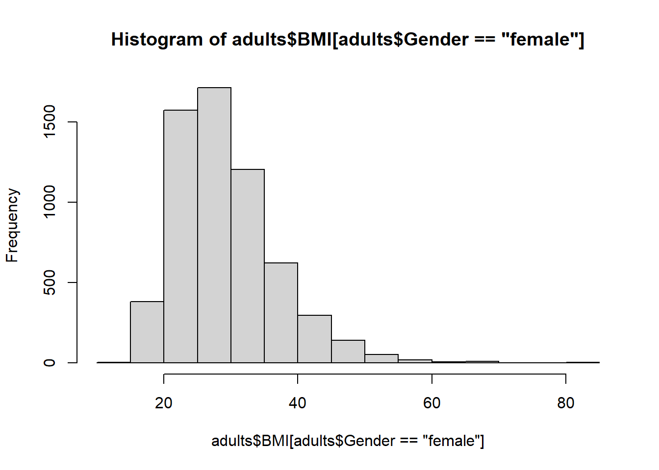
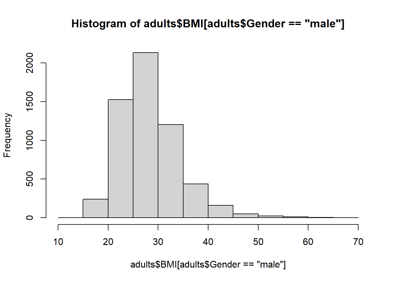
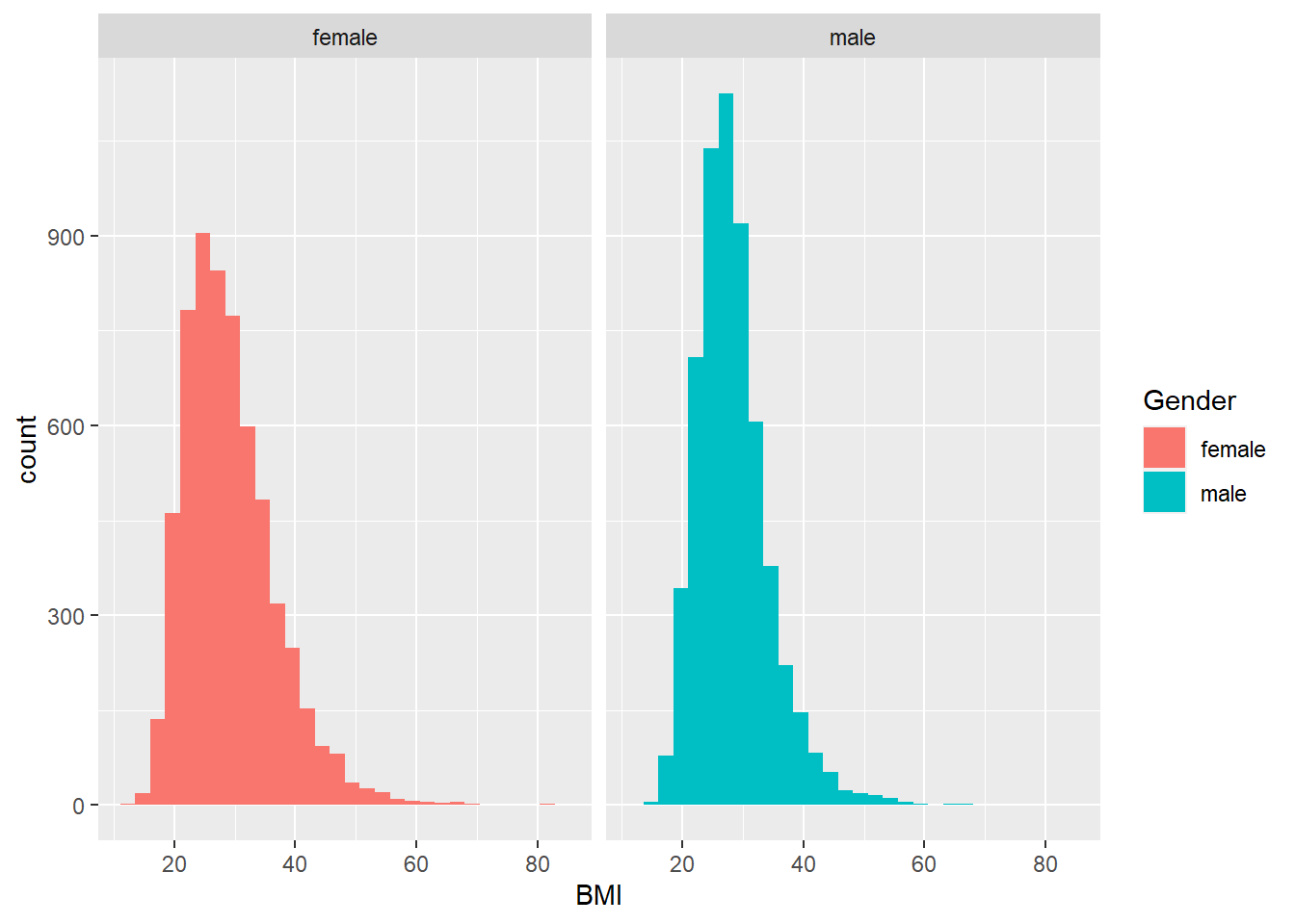
Let’s look at whether BMI differs between men and women:

hist(adults$BMI[adults$Gender=="female"])

hist(adults$BMI[adults$Gender=="male"])

Or let’s do it the ggplot2 way

# Define default colour scale suitable for colour-blind users

scale_colour_discrete <- ggthemes::scale_color_colorblind

# Create plot facetted by Gender
ggplot(adults, aes(BMI, fill = Gender)) +
  geom_histogram() +
  facet_wrap(.~Gender)

## Warning: Removed 580 rows containing non-finite values (stat_bin).

Any guesses on whether there is a significant difference? Now it’s time to do the test.

t.test(x = adults$BMI[adults$Gender == "female"],
       y = adults$BMI[adults$Gender == "male"],
       alternative = "two.sided", # could also be 'less' or 'greater' for one-sided test
       paired = FALSE) 

## 
##  Welch Two Sample t-test
## 
## data:  adults$BMI[adults$Gender == "female"] and adults$BMI[adults$Gender == "male"]
## t = 7.1026, df = 11386, p-value = 1.297e-12
## alternative hypothesis: true difference in means is not equal to 0
## 95 percent confidence interval:
##  0.6484638 1.1428217
## sample estimates:
## mean of x mean of y 
##  29.26902  28.37338

Yes, on average women seem to have a higher BMI in this survey.