Chapter 7 Plotting basic charts (base R)

It is important to distinguish between exploratory graphs and explanatory graphs: * Exploratory is done as part of analysis and there is no need to be pretty * Explanatory graphs are done once we understand the data and want to get insights across (for sharing with others)

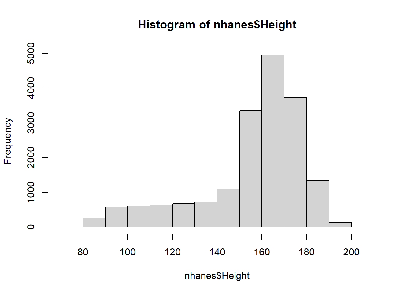
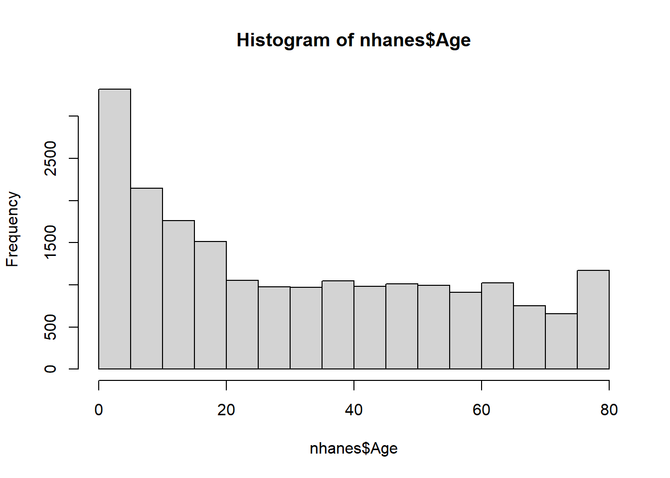
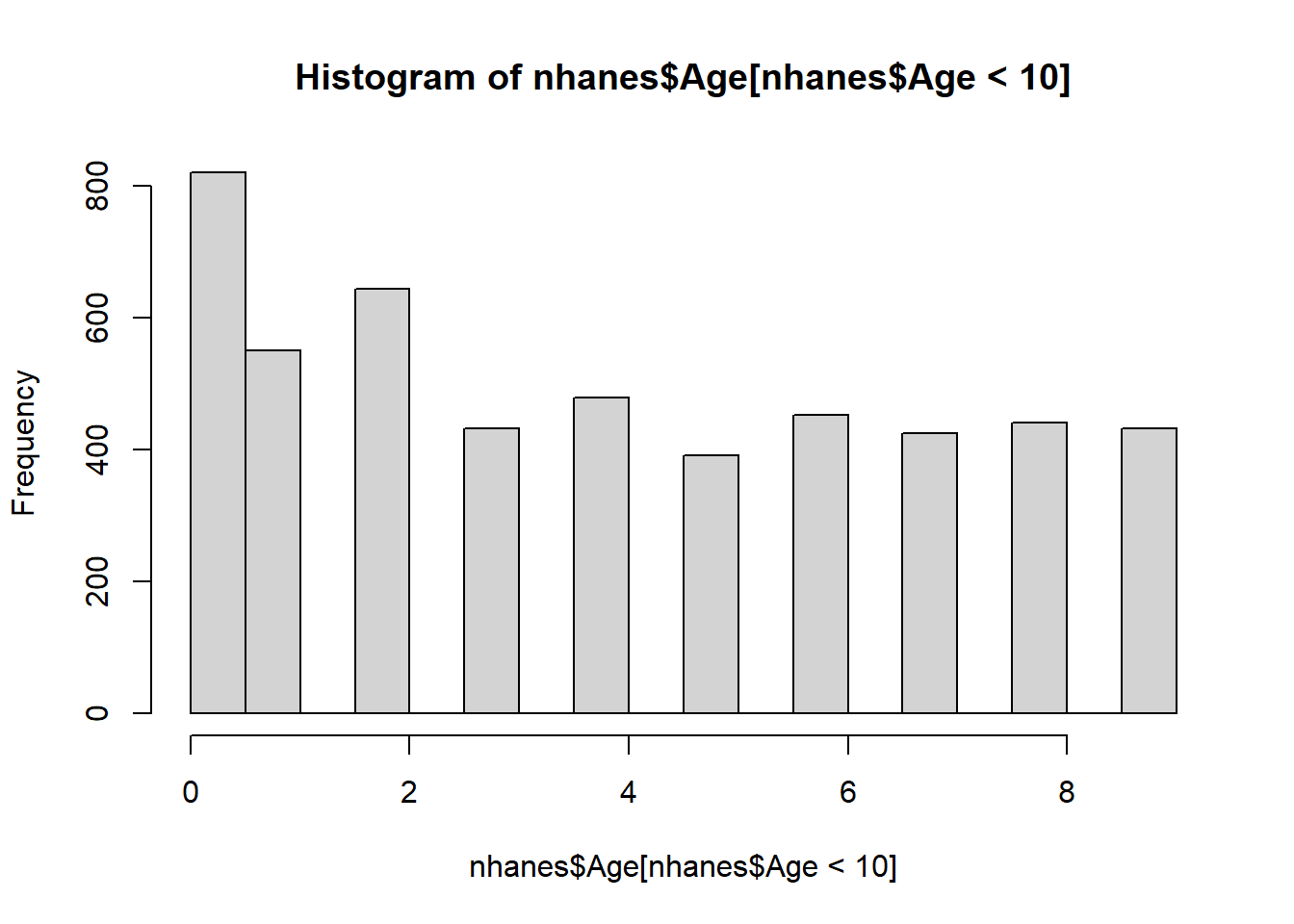
7.1 histograms - basic frequencies

# basic frequencies for numerical variables
hist(nhanes$Height)

hist(nhanes$Age)

hist(nhanes$Age[nhanes$Age<10]) # they sampled for both 0-6months and 6-12months

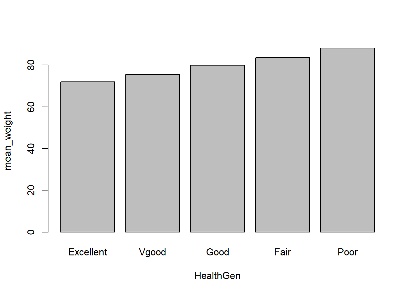
7.2 bar charts - plotting stats across categories

# Great for plotting a statistic (e.g. mean value) for categorical data
# Get dataframe into right format
aggregates_by_health <- nhanes %>% dplyr::group_by(HealthGen) %>% 
  dplyr::summarise(count = n(),
            mean_weight = round(mean(Weight, na.rm=T),1),
            mean_age = round(mean(Age, na.rm=T),1))

# create bar plot to plot either Frequencies or aggregate statistics
# Participant numbers by race
barplot(count ~ HealthGen, data = aggregates_by_health)

# average weight and age by race
barplot(mean_weight ~ HealthGen, data = aggregates_by_health)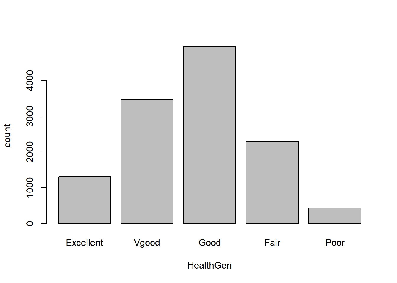

7.3 Box plots - plotting distribution of several categories/vars

# Good for distribution of continuous data across categories
boxplot(nhanes$Age ~ HealthGen, data = nhanes )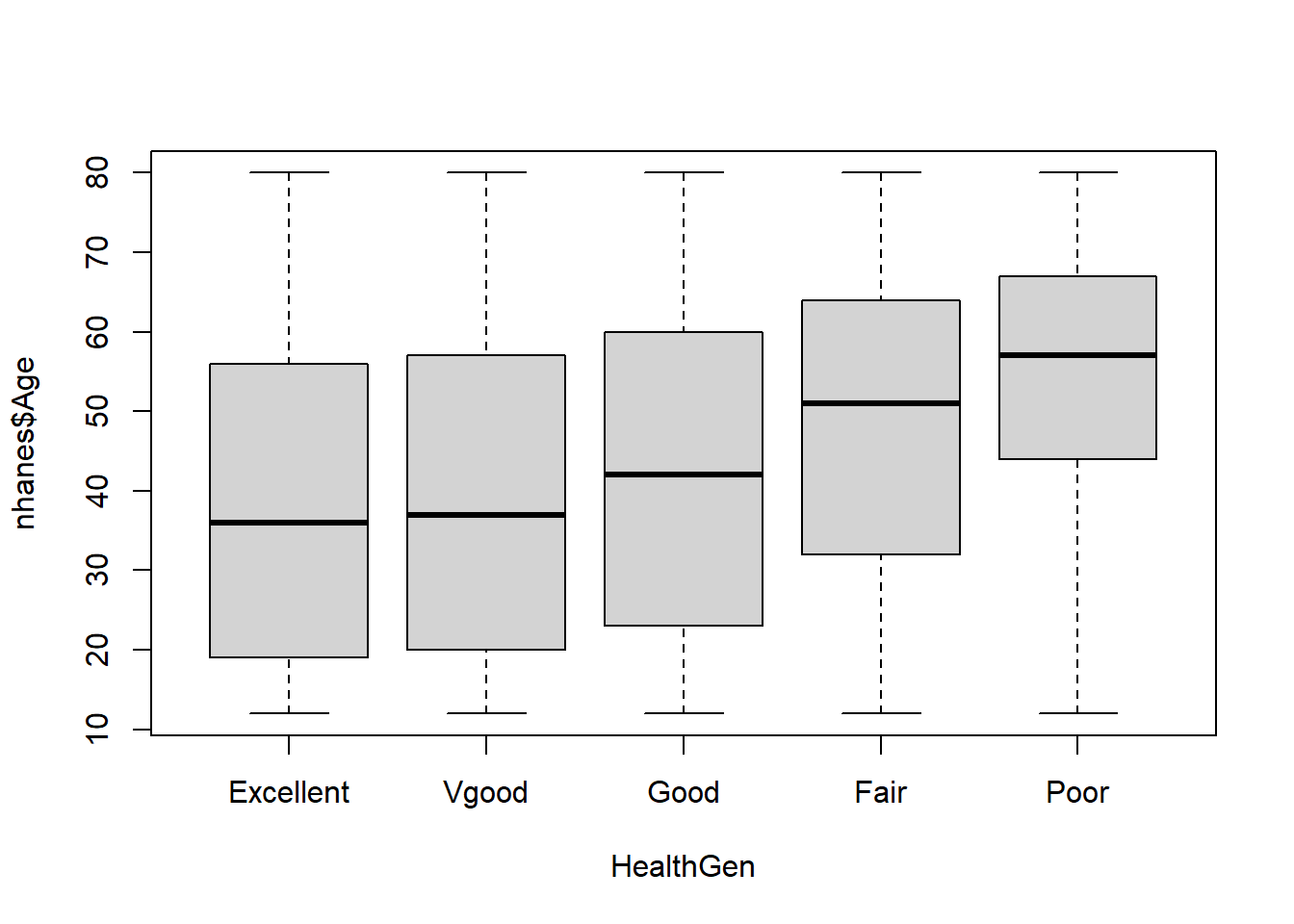

7.4 Scatter plots - relationship between two continuous vars

# Let's keep only adults in for this
adults <- nhanes %>% dplyr::filter(Age >= 18)

# plot scatter plot
plot(x = adults$Height, y = adults$Weight)

Can you guess the Correlation coefficient? What’s the value of the correlation coefficient?"

cor(adults$Height, adults$Weight, use = "pairwise.complete.obs")

## [1] 0.434507

Now let’s add the line of best fit. First, we calculate slope and intercept of line of best fit

coef(lm(Weight ~ Height, data = adults))

## (Intercept)      Height 
##  -72.209450    0.915329

Then we can add them to the plot

# add them to plot (run both commands)
plot(x = adults$Height, y = adults$Weight)
# intercept and slope
abline(-72.209450 , 0.915329)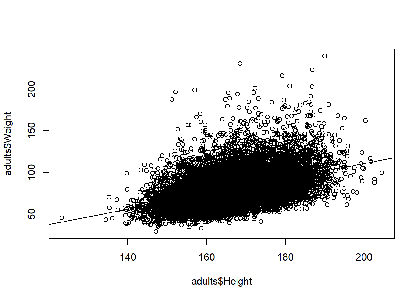

7.5 Tiny statistics excursion

What’s the relationship between the linear model regression coefficient and the correlation coefficient?

hnorm <- adults$Height/sd(adults$Height, na.rm = TRUE)
wnorm <- adults$Weight/sd(adults$Weight, na.rm = TRUE)
df_norm <- as.data.frame(cbind(hnorm,wnorm))

coef(lm(hnorm ~ wnorm, data = df_norm))

## (Intercept)       wnorm 
##  14.7794973   0.4345723

Note: For correlation coef, the larger the value, the stronger the (linear!) relationship. For regression coefficients, a larger slope coefficient does NOT imply that the association between variables is stronger (remember the unit dependency).

Intermediate R - R for Survey Analysis