4 Results of the study
library(tidyverse)
library(gtsummary)
library(psych)
library(ggstatsplot)
library(equatiomatic)
library(gt)
library(patchwork)
4.1 Introduction
The objectives of this study are to determine the perceived level of the employee’s motivation for knowledge sharing and the perceived level of the employee creativity and to investigate the relationship between the employee’s motivation for knowledge sharing and employee creativity in the Industrial Park of Jiujiang National Economic and Technology Development Zone. The questionnaires were distributed online, and 403 valid questionnaires were finally collected. The statistics used to analyze the data are Frequency, Mean, Standard Deviation, Pearson correlation, and Linear regression analysis. The tool used for data analysis is RStudio: a free software that provides open source and enterprise-ready professional software for data science.
The variables used in this chapter are:
X = Mean
SD = Standard deviation
r = Pearson correlation coefficient
p = Statistical significance
4.2 Demographic Information
- Table 4.1: Frequency and Percentage of Gender
df %>%
  mutate(gender_sort = if_else(gender == 1, "male", "female")) %>%
  select(gender_sort) %>%
  tbl_summary(
    statistic = list(gender_sort ~ "{n} ({p}%)"),
    digits = gender_sort ~ c(0, 2)
  ) %>%
modify_caption("Frequency and Percentage of Gender")| Characteristic | N = 4031 |
|---|---|
| gender_sort | |
| female | 205 (50.87%) |
| male | 198 (49.13%) |
| 1 n (%) | |
- Figure 4.1: Frequency and Percentage of Gender
df %>%
  mutate(gender_sort = if_else(gender == 1, "male", "female")) %>%
  group_by(gender_sort) %>%
  summarise(
    n = n(),
    prop = scales::label_percent(accuracy = 0.01)(n / nrow(df))
  ) %>%
  ggplot(aes(x = gender_sort, y = n, fill = gender_sort)) +
  geom_col(width = 0.3) +
  geom_text(aes(label = n), vjust = -0.2) +
  theme_clean() +
  theme(legend.position = "none")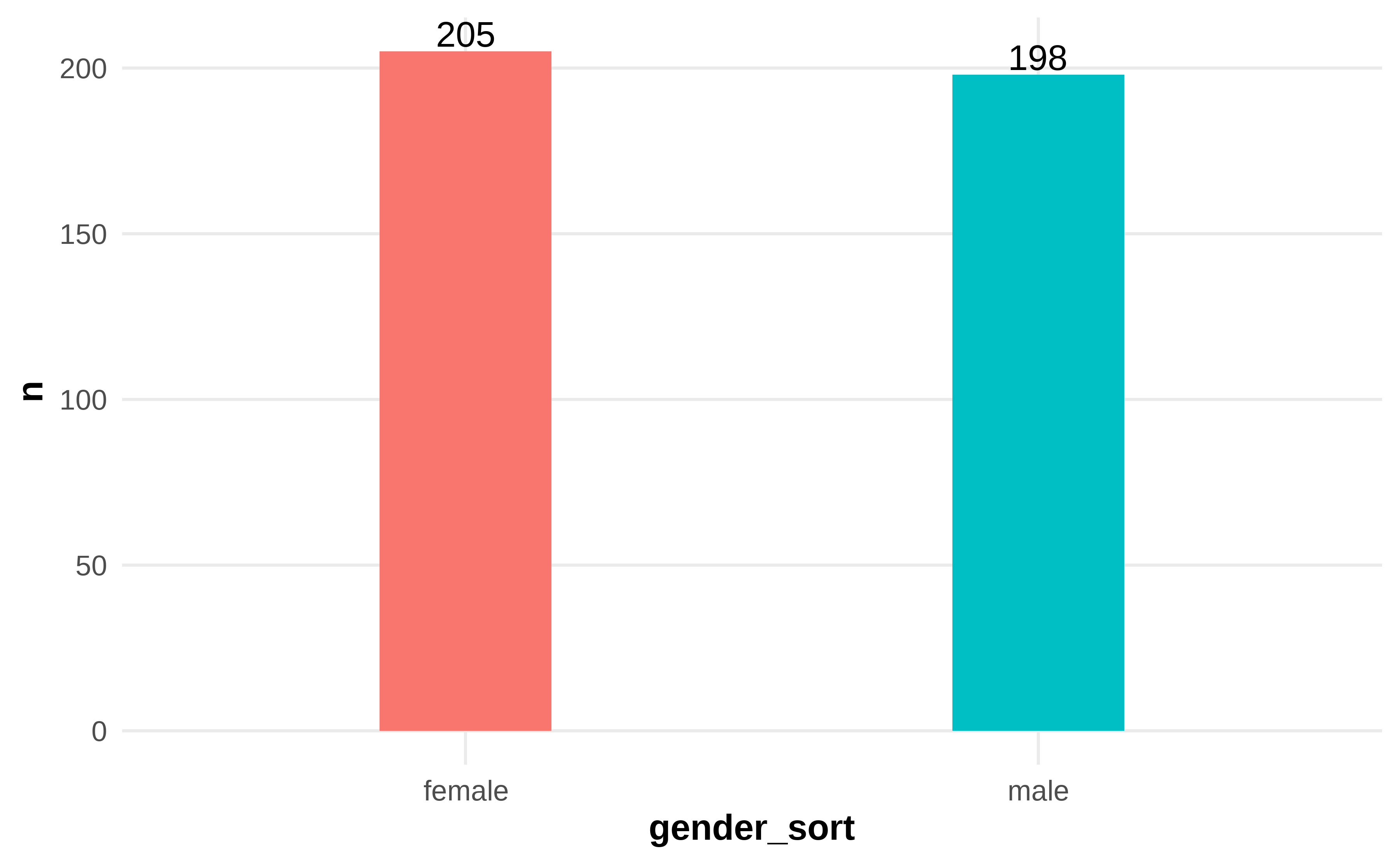
Figure 4.1: Frequency and Percentage of Gender
Table 4.1 shows 403 questionnaires, and the females are slightly more than the males. Specifically, 205 females account for 50.87%, and 198 males account for 49.13%.
- Table 4.2: Frequency and Percentage of Age
df %>%
  mutate(age_sort = case_when(
    age == 1 ~ "under 25",
    age == 2 ~ "26-35",
    age == 3 ~ "36-45",
    age == 4 ~ "above 45")) %>%
  mutate(age_sort = factor(age_sort, levels = c("under 25", "26-35", "36-45", "above 45"))) %>%
  select(age_sort) %>%
  tbl_summary(
    statistic = list(age_sort ~ "{n} ({p}%)"),
    digits = age_sort ~ c(0, 2)
    ) %>%
modify_caption("Frequency and Percentage of Age")| Characteristic | N = 4031 |
|---|---|
| age_sort | |
| under 25 | 59 (14.64%) |
| 26-35 | 158 (39.21%) |
| 36-45 | 111 (27.54%) |
| above 45 | 75 (18.61%) |
| 1 n (%) | |
- Figure 4.2: Frequency and Percentage of Age
df %>%
  mutate(age_sort = case_when(
    age == 1 ~ "under 25",
    age == 2 ~ "26-35",
    age == 3 ~ "36-45",
    age == 4 ~ "above 45"
  )) %>%
  mutate(
    age_sort = factor(age_sort, levels = c("under 25", "26-35", "36-45", "above 45"))
    ) %>%
  group_by(age_sort) %>%
  summarise(
    n = n(),
    prop = scales::label_percent(accuracy = 0.01)(n / nrow(df))
  ) %>%
  ggplot(aes(x = age_sort, y = n, fill = age_sort)) +
  geom_col(width = 0.3) +
  geom_text(aes(label = n), vjust = -0.2) +
  theme_clean() +
  theme(legend.position = "none")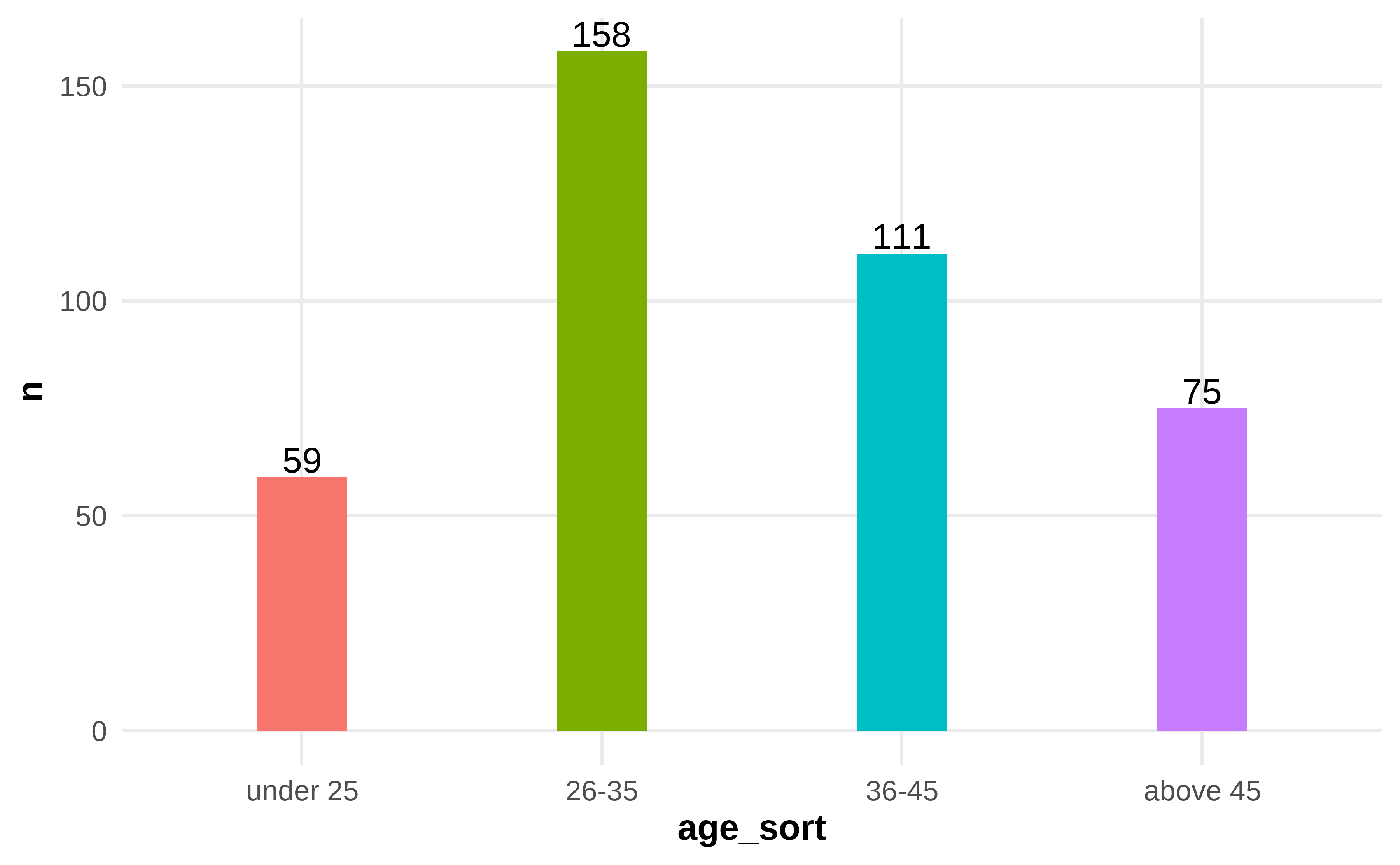
Figure 4.2: Frequency and Percentage of Age
Table 4.2 shows the age distribution according to 403 questionnaire surveys. The highest proportion is 26 to 35 years old, 158 employees account for 39.2%. Conversely, under 25 years old 59 employees account for 14.6% is the lowest, 36-45 years old 111 employees and above 46 years old 75 employees, account for 27.5% and 18.6% respectively.
- Table 4.3: Frequency and Percentage of Educational Background
df %>%
  mutate(educational_background_sort = case_when(
    educational_background == 1 ~ "high school diploma or below",
    educational_background == 2 ~ "college degree",
    educational_background == 3 ~ "bachelor degree",
    educational_background == 4 ~ "graduate or above"
  )) %>%
  mutate(
    educational_background_sort = factor(educational_background_sort, levels = c("high school diploma or below", "college degree", "bachelor degree", "graduate or above"))
  ) %>%
  select(educational_background_sort) %>%
  tbl_summary(
    statistic = list(educational_background_sort ~ "{n} ({p}%)"),
    digits = educational_background_sort ~ c(0, 2)
    ) %>%
modify_caption("Frequency and Percentage of Educational Background")| Characteristic | N = 4031 |
|---|---|
| educational_background_sort | |
| high school diploma or below | 7 (1.74%) |
| college degree | 123 (30.52%) |
| bachelor degree | 221 (54.84%) |
| graduate or above | 52 (12.90%) |
| 1 n (%) | |
- Figure 4.3: Frequency and Percentage of Educational Background
df %>%
  mutate(educational_background_sort = case_when(
    educational_background == 1 ~ "high school diploma or below",
    educational_background == 2 ~ "college degree",
    educational_background == 3 ~ "bachelor degree",
    educational_background == 4 ~ "graduate or above"
  )) %>%
  mutate(
    educational_background_sort = factor(educational_background_sort, levels = c("high school diploma or below", "college degree", "bachelor degree", "graduate or above"))
  ) %>%
  group_by(educational_background_sort) %>%
  summarise(
    n = n(),
    prop = scales::label_percent(accuracy = 0.01)(n / nrow(df))
    ) %>%
  ggplot(aes(x = educational_background_sort, y = n, fill = educational_background_sort)) +
  geom_col(width = 0.3) +
  geom_text(aes(label = n), vjust = -0.2) +
  theme_clean() +
  theme(legend.position = "none")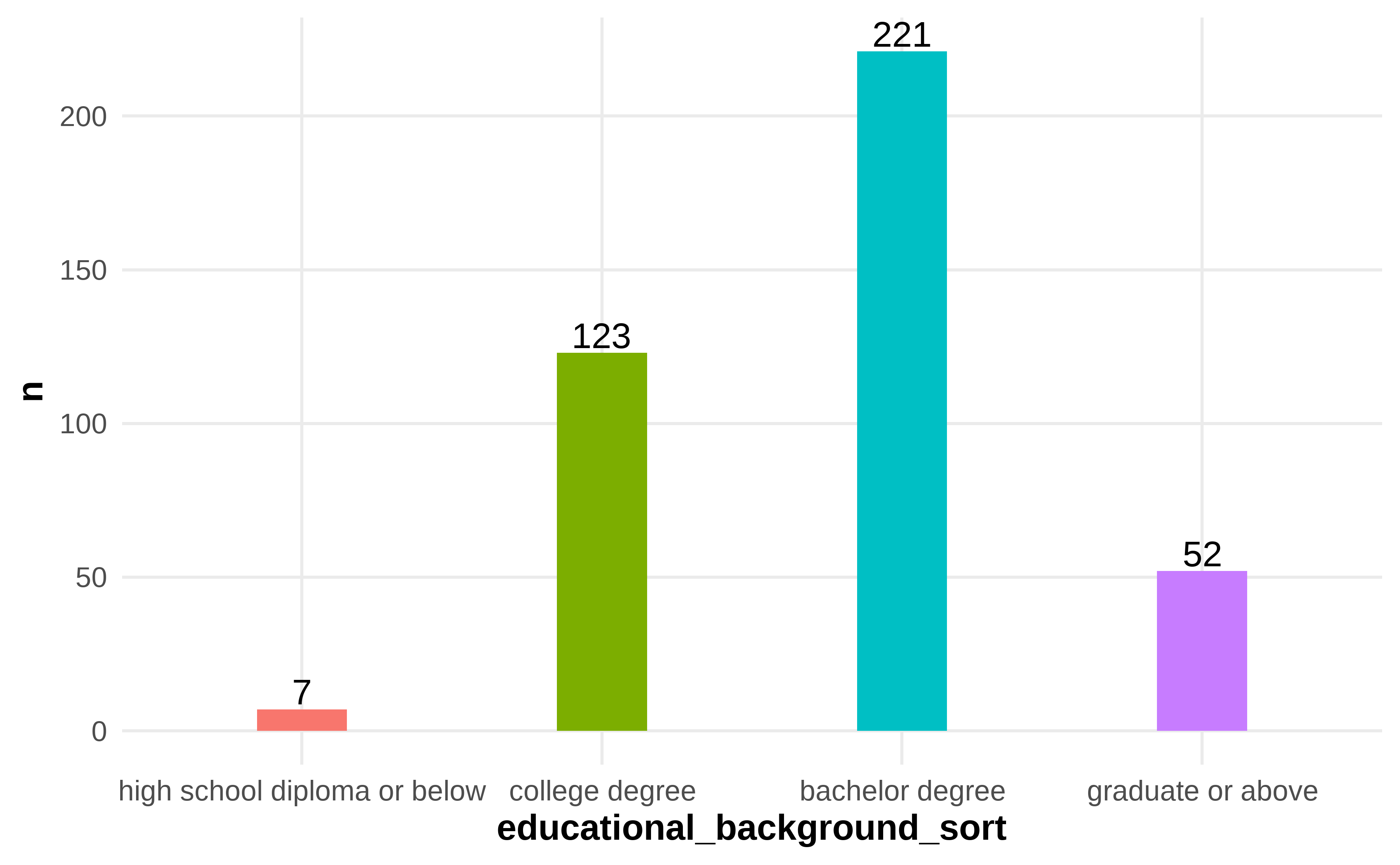
Figure 4.3: Frequency and Percentage of Educational Background
Table 4.3 shows the survey results on the educational background of respondents. Firstly, 221 people with bachelor’s degrees occupy 54.84% of the total. The next is the college degree, 123 people occupy 30.25%, 52 who have graduated or above educated occupy 12.90%, and 7 has a high school diploma or below educated occupy 1.74%.
- Table 4.4: Frequency and Percentage of Work Experience
df %>%
  mutate(work_experience_sort = case_when(
    work_experience == 1 ~ "less than 3 years",
    work_experience == 2 ~ "4-6 years",
    work_experience == 3 ~ "7-9 years",
    work_experience == 4 ~ "more than 10 years"
  )) %>%
  mutate(
    work_experience_sort = factor(work_experience_sort, levels = c("less than 3 years", "4-6 years", "7-9 years", "more than 10 years"))
  ) %>%
  select(work_experience_sort) %>%
  tbl_summary(
    statistic = list(work_experience_sort ~ "{n} ({p}%)"),
    digits = work_experience_sort ~ c(0, 2)
    ) %>%
modify_caption("Frequency and Percentage of Work Experience")| Characteristic | N = 4031 |
|---|---|
| work_experience_sort | |
| less than 3 years | 74 (18.36%) |
| 4-6 years | 118 (29.28%) |
| 7-9 years | 124 (30.77%) |
| more than 10 years | 87 (21.59%) |
| 1 n (%) | |
- Figure 4.4: Frequency and Percentage of Work Experience
df %>%
  mutate(work_experience_sort = case_when(
    work_experience == 1 ~ "less than 3 years",
    work_experience == 2 ~ "4-6 years",
    work_experience == 3 ~ "7-9 years",
    work_experience == 4 ~ "more than 10 years"
  )) %>%
  mutate(
    work_experience_sort = factor(work_experience_sort, levels = c("less than 3 years", "4-6 years", "7-9 years", "more than 10 years"))
  ) %>%
  group_by(work_experience_sort) %>%
  summarise(
    n = n(),
    prop = scales::label_percent(accuracy = 0.01)(n / nrow(df))
    ) %>%
  ggplot(aes(x = work_experience_sort, y = n, fill = work_experience_sort)) +
  geom_col(width = 0.3) +
  geom_text(aes(label = n), vjust = -0.2) +
  theme_clean() +
  theme(legend.position = "none")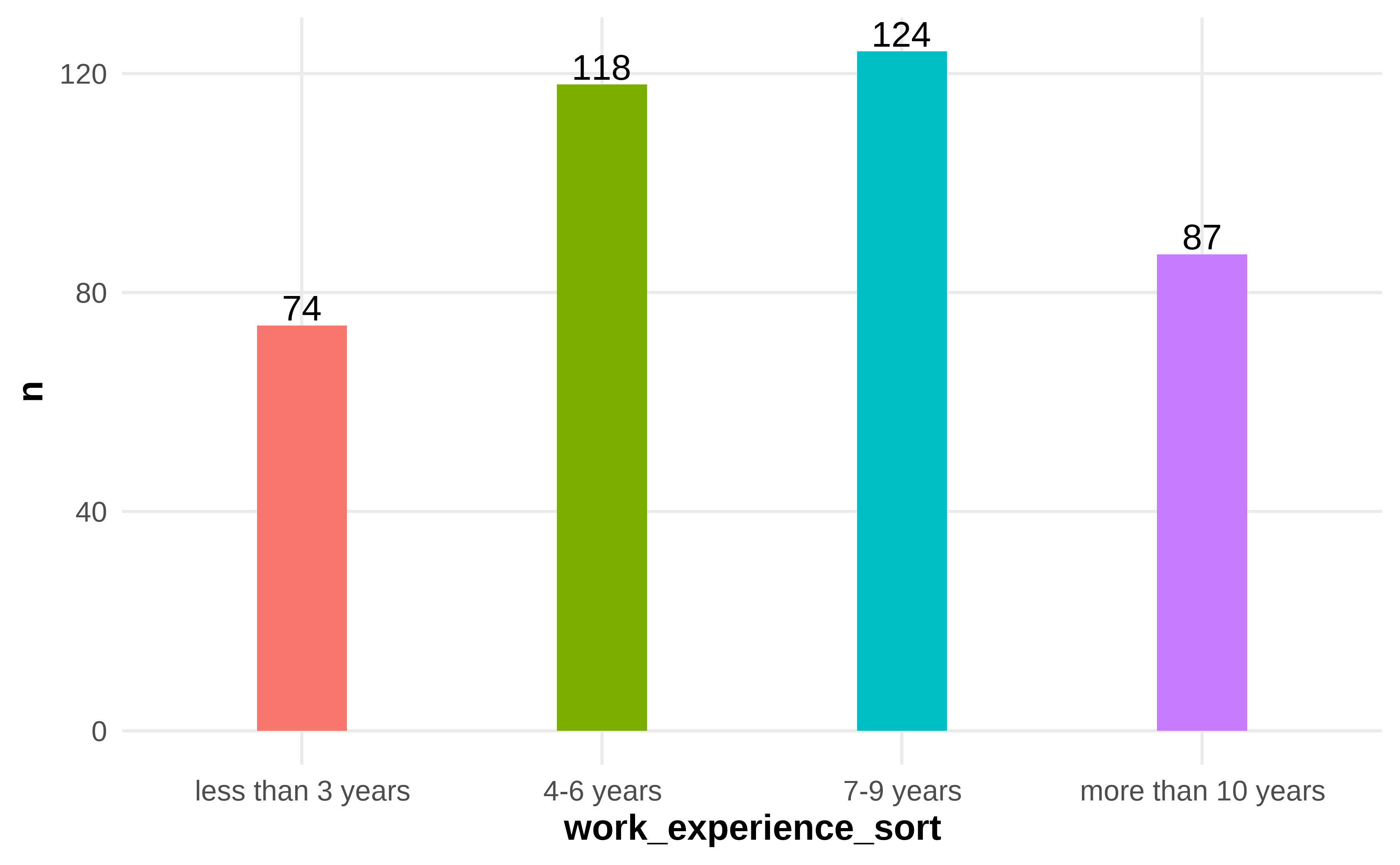
Figure 4.4: Frequency and Percentage of Work Experience
Table 4.4 shows the 403 respondents’ working experiences. Among them, 124 of whom worked for 7-9 years, which is the highest proportion, account for 30.77%, followed by the group who worked for 4-6 years, 118 people account for 29.28%, 87 worked for more than 10 years, accounts for 21.59%, and 74 worked for less than 3 years accounts for 18.36%.
- Table 4.5: Frequency and Percentage of Position Level
df %>%
  mutate(position_level_sort = case_when(
    position_level == 1 ~ "general staff",
    position_level == 2 ~ "first-line manager",
    position_level == 3 ~ "middle manager",
    position_level == 4 ~ "top manager"
  )) %>%
  mutate(
    position_level_sort = factor(position_level_sort, levels = c("general staff", "first-line manager", "middle manager", "top manager"))
  ) %>%
 select(position_level_sort) %>%
  tbl_summary(
    statistic = list(position_level_sort ~ "{n} ({p}%)"),
    digits = position_level_sort ~ c(0, 2)
    ) %>%
modify_caption("Frequency and Percentage of Position Level")| Characteristic | N = 4031 |
|---|---|
| position_level_sort | |
| general staff | 295 (73.20%) |
| first-line manager | 54 (13.40%) |
| middle manager | 30 (7.44%) |
| top manager | 24 (5.96%) |
| 1 n (%) | |
- Figure 4.5: Frequency and Percentage of Position Level
df %>%
  mutate(position_level_sort = case_when(
    position_level == 1 ~ "general staff",
    position_level == 2 ~ "first-line manager",
    position_level == 3 ~ "middle manager",
    position_level == 4 ~ "top manager"
  )) %>%
  mutate(
    position_level_sort = factor(position_level_sort, levels = c("general staff", "first-line manager", "middle manager", "top manager"))
  ) %>%
  group_by(position_level_sort) %>%
  summarise(
    n = n(),
    prop = scales::label_percent(accuracy = 0.01)(n / nrow(df))
  ) %>%
  ggplot(aes(x = position_level_sort, y = n, fill = position_level_sort)) +
  geom_col(width = 0.3) +
  geom_text(aes(label = n), vjust = -0.2) +
  theme_clean() +
  theme(legend.position = "none")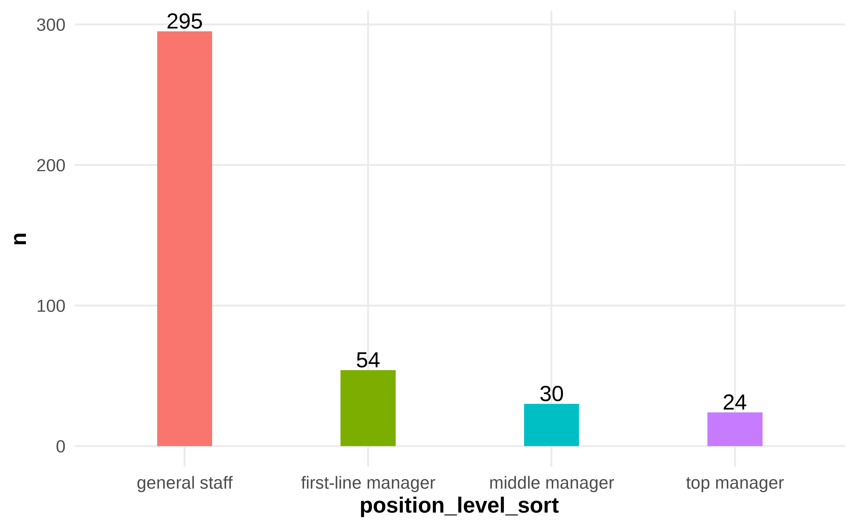
Figure 4.5: Frequency and Percentage of Position Level
Table 4.5 shows 403 survey results of position level in respondents. Specifically, 295 general staff account for 73.20% are the most part, 54 first-line managers account for 13.40%, 30 middle managers account for 7.44%, and 24 top managers account for 5.96%.
4.3 Results of the Study
d1 <- df %>%
  rowwise() %>%
  mutate(
    f_achievement = mean(c_across(cols = starts_with("a_achievement"))),
    f_collectivity = mean(c_across(cols = starts_with("a_collectivity"))),
    f_social = mean(c_across(cols = starts_with("a_social"))),
    f_interest = mean(c_across(cols = starts_with("a_interest"))),
    f_rule = mean(c_across(cols = starts_with("a_rule"))),
    a = mean(c_across(cols = starts_with("a_"))),
    b = mean(c_across(cols = starts_with("b_")))
) %>%
  ungroup()
4.3.1 Descriptive Statistical Analysis
- Table 4.6: Mean & SD of Total Employee’s Motivation for Knowledge Sharing
d1 %>%
  select(starts_with("f_"), a) %>%
  tbl_summary(statistic =  everything() ~ "{mean} ({sd})") %>%
modify_caption("Mean & SD of Total Employee's Motivation for Knowledge Sharing")| Characteristic | N = 4031 |
|---|---|
| f_achievement | 4.38 (0.75) |
| f_collectivity | 4.28 (0.85) |
| f_social | 4.39 (0.73) |
| f_interest | 4.33 (0.81) |
| f_rule | 4.20 (0.91) |
| a | 4.33 (0.73) |
| 1 Mean (SD) | |
Table 4.6 shows that the employee’s motivation for knowledge sharing is at an agreed level, X = 4.33, SD = 0.73. Meanwhile, all aspects of the employee’s motivation for knowledge sharing have a wide return at an agreed level. The highest is the aspect of construction of social relations, X = 4.39, SD = 0.73. The second level is the aspect of the perception of achievement, X = 4.38, SD = 0.75. The aspect of personal interest is the third, X = 4.33, SD = 0.81. The aspect of collective emotions and responsibilities is the next, X = 4.28, SD = 0.85. The last one is the aspect of rule obedience, X = 4.20, SD = 0.91.
- Table 4.7: Mean & SD of The Perception of Achievement
d1 %>%
  select(contains("achievement")) %>%
  tbl_summary(statistic = list(everything() ~ "{mean} ({sd})"),
              type = list(everything() ~ 'continuous')) %>%
modify_caption("Mean & SD of The Perception of Achievement")| Characteristic | N = 4031 |
|---|---|
| a_achievement_recognized | 4.39 (0.78) |
| a_achievement_praised | 4.33 (0.84) |
| a_achievement_respected | 4.35 (0.84) |
| a_achievement_value | 4.45 (0.79) |
| f_achievement | 4.38 (0.75) |
| 1 Mean (SD) | |
Table 4.7 shows that the perception of achievement, one aspect of the employee’s motivation for knowledge sharing, is at an agreed level, X = 4.38, SD = 0.75, as mentioned above. All aspects of perception of achievement have a total return at an agreed level. The highest level is “I think contributing knowledge and sharing experience reflect my achievements and value,” X = 4.45, SD = 4.39. The second is “I think contributing knowledge to colleagues helps be more recognized,” X = 4.39, SD = 0.78. “I think contributing knowledge to colleagues helps be more respected” is the next, X = 4.35, SD = 0.79. The fourth is “I think contributing knowledge to colleagues helps be more praised,” X = 4.33, SD = 0.84.
- Table 4.8: Mean & SD of Collective Emotions and Responsibilities
d1 %>%
  select(contains("collectivity")) %>%
  tbl_summary(statistic = list(everything() ~ "{mean} ({sd})"),
              type = list(everything() ~ 'continuous')) %>%
modify_caption("Mean & SD of Collective Emotions and Responsibilities")| Characteristic | N = 4031 |
|---|---|
| a_collectivity_congtribution | 4.38 (0.82) |
| a_collectivity_paticipantion | 4.36 (0.87) |
| a_collectivity_responsibility | 4.10 (1.07) |
| f_collectivity | 4.28 (0.85) |
| 1 Mean (SD) | |
Table 4.8 shows the collective emotions and responsibilities: one aspect of the employee’s motivation for knowledge sharing is at an agreed level, as is shown in table 4.6, X = 4.28, SD = 0.85. In the meantime, all aspects of collective emotions and responsibilities are at the agreed level. More detailed, the highest level of collective emotions and responsibilities is “I contribute my knowledge and share my experience with the organization because I love it,” X = 4.38, SD = 0.82. “I participate in knowledge-sharing activities because I love my organization,” X = 4.36, SD = 0.87, ranked second. “It’s my responsibility to contribute my knowledge and share experience with the organization or colleagues,” X = 4.10, SD = 1.07 ranked last in this aspect.
- Table 4.9: Mean & SD of Construction of Social Relations
d1 %>%
  select(contains("social")) %>%
  tbl_summary(statistic = list(everything() ~ "{mean} ({sd})"),
              type = list(everything() ~ 'continuous')) %>%
modify_caption("Mean & SD of Construction of Social Relations")| Characteristic | N = 4031 |
|---|---|
| a_social_identification | 4.33 (0.84) |
| a_social_range | 4.39 (0.77) |
| a_social_acquaintance | 4.41 (0.76) |
| a_social_friendship | 4.40 (0.78) |
| a_social_connection | 4.40 (0.79) |
| f_social | 4.39 (0.73) |
| 1 Mean (SD) | |
Table 4.9 shows that the construction of the social relations, an aspect of the employee’s motivation for knowledge sharing, is at an agreed level, as is shown in table 4.6, X = 4.39, SD = 0.73. Meanwhile, five aspects of the construction of social relations are at the agreed level. The highest level is “Contributing my knowledge, and sharing experience with others makes me more acquainted with other organization members,” X = 4.41, SD = 0.76. “Contributing my knowledge and sharing experience with others can promote our friendship and feelings” is followed, X = 4.40, SD = 0.78. The next, “Contributing my knowledge and sharing experience can strengthen your bonds with others,” X = 4.40, SD = 0.79. The fourth, “Contributing my knowledge and sharing experience can strengthen your bonds with others,” X = 4.39, SD = 0.73. Lastly, “Contributing my knowledge and sharing experience to the organization can enhance colleagues’ identification with me,” X = 4.33, SD = 0.84.
- Table 4.10: Mean & SD of Personal Interest
d1 %>%
  select(contains("interest")) %>%
  tbl_summary(statistic = list(everything() ~ "{mean} ({sd})"),
              type = list(everything() ~ 'continuous')) %>%
modify_caption("Mean & SD of Personal Interest")| Characteristic | N = 4031 |
|---|---|
| a_interest_interesting | 4.35 (0.82) |
| a_interest_pleasant | 4.37 (0.83) |
| a_interest_enjoyed | 4.25 (0.90) |
| f_interest | 4.33 (0.81) |
| 1 Mean (SD) | |
Table 4.10 shows that the personal interest, an aspect of the employee’s motivation for knowledge sharing, is at an agreed level, X = 4.33, SD = 0.81. All three factors involved in the personal interest are at the agreed level. The highest one is “I think it’s pleasant to share my knowledge and experience with my colleagues,” X = 4.37, SD = 0.83. The second is “I think it’s interesting to share my knowledge and experience with my colleagues,” X = 4.35, SD = 0.82. The third one is “I enjoy sharing my work experience and skills with colleagues very much,” X = 4.25, SD = 0.90.
- Table 4.11: Mean & SD of Rule Obedience
d1 %>%
  select(contains("rule")) %>%
  tbl_summary(statistic = list(everything() ~ "{mean} ({sd})"),
              type = list(everything() ~ 'continuous')) %>%
modify_caption("Mean & SD of Rule Obedience")| Characteristic | N = 4031 |
|---|---|
| a_rule_obedience | 4.17 (1.01) |
| a_rule_ethical | 4.08 (1.12) |
| a_rule_conscious | 4.34 (0.85) |
| f_rule | 4.20 (0.91) |
| 1 Mean (SD) | |
Table 4.11 shows the aspect of employee’s motivation for knowledge sharing, the rule obedience, is at an agreed level, X = 4.2, SD = 0.91. Specifically, “If contributing knowledge is a rule in my organization, and I’ll try to abide by it” is the highest score, X = 4.34, SD = 0.85. Then “If contributing knowledge is a collective rule or regulation, all members should abide by it” is the second, X = 4.17, SD = 1.01. The last one is “It’s unethical to violate the collective rule or regulation of sharing knowledge,” X = 4.08, SD = 1.02.
- Table 4.12: Mean & SD of Total Employee Creativity
d1 %>%
  select(starts_with("b")) %>%
  tbl_summary(statistic = list(everything() ~ "{mean} ({sd})"),
              type = list(everything() ~ 'continuous')) %>%
modify_caption("Mean & SD of Total Employee Creativity")| Characteristic | N = 4031 |
|---|---|
| b_goal | 4.27 (0.81) |
| b_performance | 4.33 (0.82) |
| b_searching | 4.35 (0.81) |
| b_improvement | 4.34 (0.82) |
| b_source | 4.36 (0.81) |
| b_risk | 3.88 (1.11) |
| b_support | 4.02 (1.06) |
| b_timly | 4.29 (0.83) |
| b_planned | 4.20 (0.95) |
| b_novel | 4.22 (0.93) |
| b_creative | 4.27 (0.87) |
| b_solution | 4.28 (0.88) |
| b_execution | 4.27 (0.87) |
| b | 4.24 (0.76) |
| 1 Mean (SD) | |
Table 4.12 shows the total employee creativity is at an agreed level, X = 4.24, SD = 0.76. As employee creativity is a unidimensional variable, we got the average perceived level of respondents based on the questionnaire results about each question on the employee creativity scale. The highest one is “It is an excellent source of ideas”, X = 4.36, SD = 0.81. Next is “Search for new science, procedures, technologies, and products ideas”, X = 4.35, SD = 0.81. No.3 is “Propose new methods to improve quality”, X = 4.34, SD = 0.82. No.4 is “Propose new practical ideas to improve performance”, X = 4.33, SD = 0.82. The last one is “Not afraid to take risks,” X = 3.88, SD = 1.11. In general, respondents perceived level of employee creativity is at the agreed-upon level.
4.3.2 Inferential Statistical Analysis
4.3.2.1 One-Sample t-test
- Table 4.13: One Sample t-test for Employee Creativity
t.test(d1$b, mu = 3, alternative = "greater") %>%
  broom::tidy() %>%
knitr::kable(caption = "One Sample t-test for Employee Creativity")| estimate | statistic | p.value | parameter | conf.low | conf.high | method | alternative |
|---|---|---|---|---|---|---|---|
| 4.24 | 32.6 | 0 | 402 | 4.17 | Inf | One Sample t-test | greater |
Table 4.13 shows the result of a one-sample t-test for employee creativity, and its result is consistent with the result in Table 4.12: the total employee creativity is at an agreed level as its mean is 4.24, greater than 3. Meanwhile, p = 4.9e-115 indicates that the result is positive and statistically significant.
4.3.2.2 Independent Samples t-test
- Table 4.14: Independent Samples t-test for Gender
t.test(total ~ gender, data = d1, var.equal = TRUE) %>%
  broom::tidy() %>%
knitr::kable(caption = "Independent Samples t-test for Gender")| estimate | estimate1 | estimate2 | statistic | p.value | parameter | conf.low | conf.high | method | alternative |
|---|---|---|---|---|---|---|---|---|---|
| 5.21 | 136 | 130 | 2.37 | 0.018 | 401 | 0.88 | 9.53 | Two Sample t-test | two.sided |
To test the significance of gender on statistical results, Table 4.14 shows that the mean total score of the male is 135.6, and the mean total score of the female is 130.4. That is to say, a true difference in means between the male and group the female is not equal to 0. According to the mean score of gender and p-value, it can be inferred that gender significantly affects the employee’s motivation for knowledge sharing and employee creativity; thus, hypothesis 1-1 and hypothesis 2-1 are supported.
4.3.2.3 One-Way ANOVA
- Table 4.15: One-Way ANOVA for Age, Educational Background, Work Experience, and Position Level
d1 %>%
  select(age:position_level, total) %>%
  tbl_uvregression(
    method = aov,
    y = total,
    pvalue_fun = function(x) style_pvalue(x, digits = 3)
  ) %>%
modify_caption("One-Way ANOVA for Age, Educational Background, Work Experience, and Position Level")| Characteristic | N | p-value |
|---|---|---|
| age | 403 | 0.239 |
| educational_background | 403 | 0.141 |
| work_experience | 403 | 0.646 |
| position_level | 403 | 0.005 |
On statistical results, as Table 4.15 shows, one-way ANOVA tests the significance of each demographic variable, including age, education background, work experience, and position level. We can infer the statistical results are not significant for age, education background, and work experience. Conversely, position level is statistically significant, which means it affects the employee’s motivation for knowledge sharing and employee creativity significantly and largely. Thus, hypothesis 1-2, hypothesis 1-3, hypothesis 1-4, hypothesis 2-2, hypothesis 2-3 and hypothesis 2-4 are not supported. Meanwhile, hypothesis 1-5 and hypothesis 2-5 are supported.
4.3.3 Pearson Correlation Analysis
- Table 4.16: Pearson Correlation Analysis on the Employee’s Motivation for Knowledge Sharing and Employee Creativity
d1 %>%
  select(f_achievement:b) %>%
  ggcorrmat(output = "dataframe",
            matrix.type = "lower",
            type = "parametric",
            sig.level = 0.05) %>%
knitr::kable(caption = "Pearson Correlation Analysis")| parameter1 | parameter2 | estimate | conf.level | conf.low | conf.high | statistic | df.error | p.value | method | n.obs |
|---|---|---|---|---|---|---|---|---|---|---|
| f_achievement | f_collectivity | 0.761 | 0.95 | 0.717 | 0.799 | 23.5 | 401 | 0 | Pearson correlation | 403 |
| f_achievement | f_social | 0.828 | 0.95 | 0.795 | 0.857 | 29.6 | 401 | 0 | Pearson correlation | 403 |
| f_achievement | f_interest | 0.771 | 0.95 | 0.728 | 0.808 | 24.3 | 401 | 0 | Pearson correlation | 403 |
| f_achievement | f_rule | 0.686 | 0.95 | 0.631 | 0.735 | 18.9 | 401 | 0 | Pearson correlation | 403 |
| f_achievement | a | 0.892 | 0.95 | 0.870 | 0.910 | 39.4 | 401 | 0 | Pearson correlation | 403 |
| f_achievement | b | 0.718 | 0.95 | 0.667 | 0.762 | 20.6 | 401 | 0 | Pearson correlation | 403 |
| f_collectivity | f_social | 0.820 | 0.95 | 0.785 | 0.850 | 28.7 | 401 | 0 | Pearson correlation | 403 |
| f_collectivity | f_interest | 0.849 | 0.95 | 0.819 | 0.874 | 32.2 | 401 | 0 | Pearson correlation | 403 |
| f_collectivity | f_rule | 0.790 | 0.95 | 0.750 | 0.824 | 25.8 | 401 | 0 | Pearson correlation | 403 |
| f_collectivity | a | 0.917 | 0.95 | 0.900 | 0.931 | 46.0 | 401 | 0 | Pearson correlation | 403 |
| f_collectivity | b | 0.787 | 0.95 | 0.746 | 0.821 | 25.5 | 401 | 0 | Pearson correlation | 403 |
| f_social | f_interest | 0.878 | 0.95 | 0.854 | 0.899 | 36.8 | 401 | 0 | Pearson correlation | 403 |
| f_social | f_rule | 0.758 | 0.95 | 0.714 | 0.797 | 23.3 | 401 | 0 | Pearson correlation | 403 |
| f_social | a | 0.946 | 0.95 | 0.935 | 0.955 | 58.5 | 401 | 0 | Pearson correlation | 403 |
| f_social | b | 0.818 | 0.95 | 0.783 | 0.848 | 28.5 | 401 | 0 | Pearson correlation | 403 |
| f_interest | f_rule | 0.806 | 0.95 | 0.769 | 0.838 | 27.3 | 401 | 0 | Pearson correlation | 403 |
| f_interest | a | 0.937 | 0.95 | 0.924 | 0.948 | 53.9 | 401 | 0 | Pearson correlation | 403 |
| f_interest | b | 0.839 | 0.95 | 0.807 | 0.865 | 30.8 | 401 | 0 | Pearson correlation | 403 |
| f_rule | a | 0.877 | 0.95 | 0.853 | 0.898 | 36.6 | 401 | 0 | Pearson correlation | 403 |
| f_rule | b | 0.758 | 0.95 | 0.713 | 0.797 | 23.3 | 401 | 0 | Pearson correlation | 403 |
| a | b | 0.856 | 0.95 | 0.828 | 0.880 | 33.2 | 401 | 0 | Pearson correlation | 403 |
- Figure 4.6: Pearson Correlation Analysis on the Employee’s Motivation for Knowledge Sharing and Employee Creativity
d1 %>%
  select(f_achievement:b) %>%
  ggcorrmat(output = "plot",
            matrix.type = "lower",
            type = "parametric",
            sig.level = 0.05,
            colors = c("#E69F00", "white", "#009E73")) +
  theme_clean()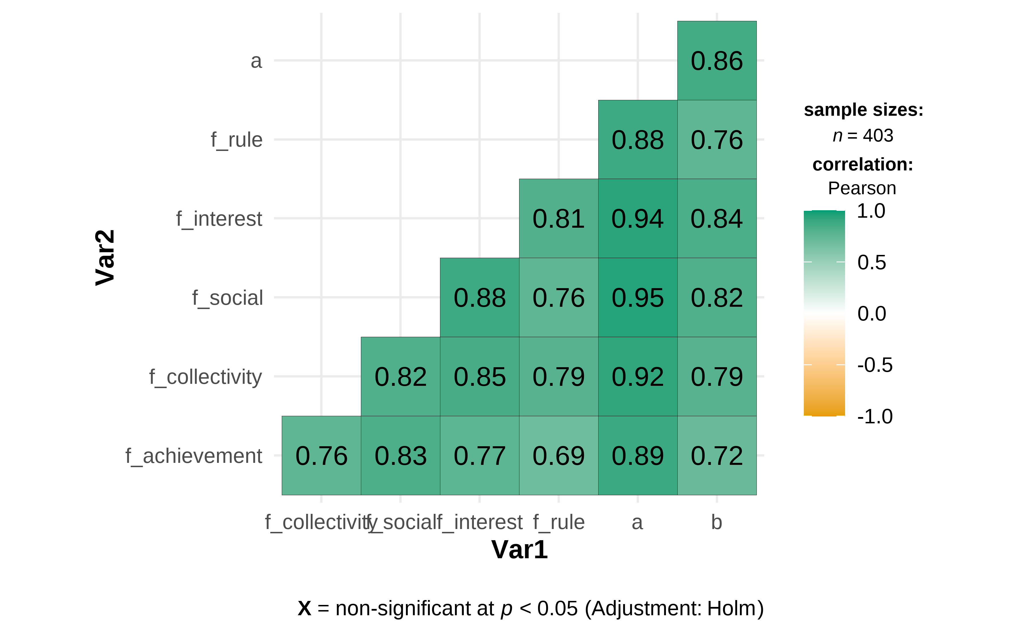
Figure 4.6: Pearson Correlations Analysis
Table 4.16 shows the statistical results on the employee’s motivation for knowledge sharing and employee creativity. In addition, Figure 4.6 is a Pearson Correlation Matrix. According to the results, there is a very strong positive correlation between the employee’s motivation for knowledge sharing and employee creativity, r = 0.86, p < 0.05. At the same time, a very strong positive correlation between personal interest and employee creativity, r = 0.84, p < 0.05, and a very strong positive correlation between the construction of the social relations and employee creativity, r = 0.82, p < 0.05. In addition, there is a strong positive correlation between the collective emotions and responsibilities and employee creativity, r = 0.79, p < 0.05. The correlation between rule obedience and employee creativity is also strong, r = 0.76, p < 0.05. The correlation coefficient between the perception of achievement and employee creativity is 0.72, and the p-value is less than 0.05, a strong positive correlation as well. Meanwhile, through testing the statistical significance of Pearson Correlation, the p-value shows that the correlation between the employee’s motivation for knowledge sharing and employee creativity is statistically significant.
4.3.4 Exploratory Factor Analysis
The employee’s motivation for knowledge sharing scale contains 18 items. Exploratory factor analysis is conducted for data dimension reduction to describe and explain the correlation among these observed variables parsimoniously.
- Data standardization and select the appropriate variables for factor analysis
df_factor <- df %>%
  mutate(across(
    starts_with("a_"), ~ (.x - mean(.x)/sd(.x))
  )) %>%
select(starts_with("a_"))- KMO and Bartlett’s test
KMO(df_factor)## Kaiser-Meyer-Olkin factor adequacy
## Call: KMO(r = df_factor)
## Overall MSA = 0.96
## MSA for each item =
## a_achievement_recognized a_achievement_praised a_achievement_respected
## 0.96 0.95 0.96
## a_achievement_value a_collectivity_congtribution a_collectivity_paticipantion
## 0.98 0.94 0.93
## a_collectivity_responsibility a_social_identification a_social_range
## 0.97 0.98 0.96
## a_social_acquaintance a_social_friendship a_social_connection
## 0.95 0.96 0.96
## a_interest_interesting a_interest_pleasant a_interest_enjoyed
## 0.95 0.94 0.96
## a_rule_obedience a_rule_ethical a_rule_conscious
## 0.94 0.94 0.97
bartlett.test(df_factor)##
## Bartlett test of homogeneity of variances
##
## data: df_factor
## Bartlett's K-squared = 187, df = 17, p-value <2e-16The KMO value of the employee’s motivation for knowledge sharing scale is 0.96, which indicates that these variables are marvelous for factor analysis. In the meantime, the chi-square value of Bartlett’s test is 187, the degree of freedom is 17, and the p-value is less than 0.05. It also suggests that all the variables are suitable for factor analysis.
- Figure 4.7: The parallel analysis
fa.parallel(df_factor)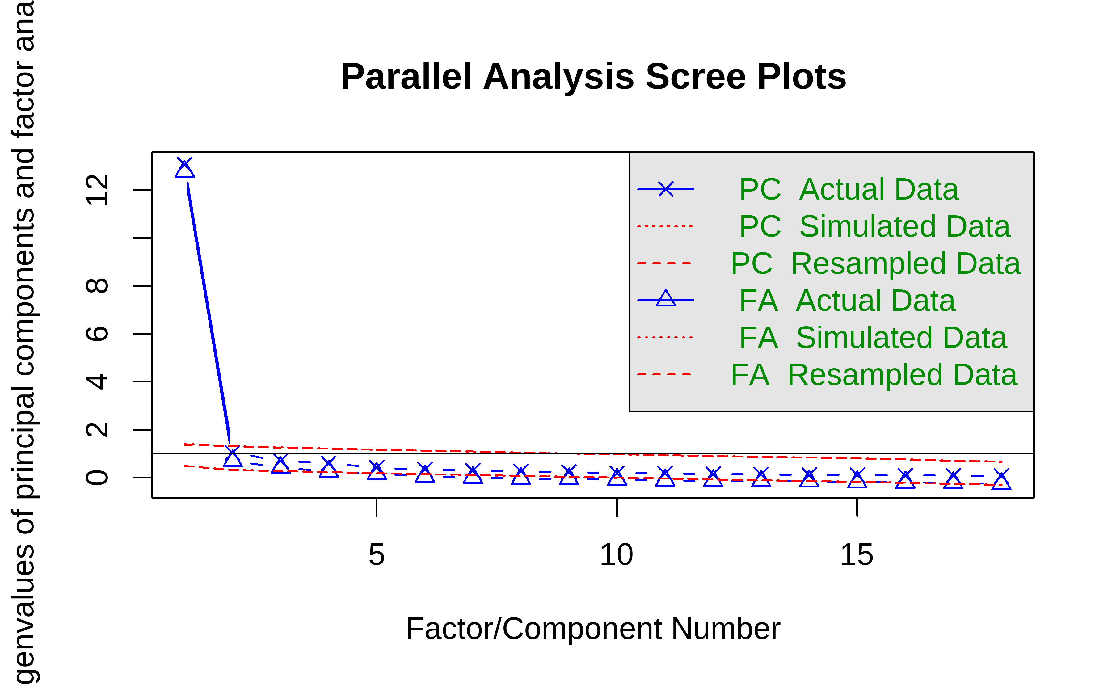
Figure 4.7: Parallel Analysis Scree Plots
## Parallel analysis suggests that the number of factors = 3 and the number of components = 1The result of parallel analysis, see Figure 4.7, illustrates that three common factors for EFA are sufficient to explain the correlation and variance among all the variables. At the same time, there are five factors with eigenvalues greater than one. To retain as much information as possible about the original variables and to ensure the explanatory power greater than 80%, the author intends to extract five common factors. Thus, the EFA model is set as Mod1 (see Equation (4.1).
\[\begin{align*} Y_{j} = l_{j1}F_{1} + l_{j2}F_{2} + l_{j3}F_{3} + l_{j4}F_{4} + l_{j5}F_{5} + \epsilon_{j} (j = 1, 2...18) \tag{4.1} \end{align*}\]
where \(Y_{j}(j = 1, 2...18)\) is a \(403\times1\) vector of observed variable score, \(F\) is a \(5\times1\) vector of common factor score, \(l_{jk}(k = 1, 2...5)\) is a \(403\times5\) matrix of factor loading that indicates the relation between the j-th observed variable and the k-th latent common factor, and \(\epsilon_{j}\) is a \(403\times1\) vector of unique factor score.
- Mod1: The EFA model of the Employee’s Motivation for Knowledge Sharing, see Equation (4.1)
Factors with eigenvalues greater than 1 are extracted by the principal component method. Factor rotation is performed by the maximum variance method. The way to do latent variable exploratory factor analysis is to use ordinary least squares to find the minimum residual solution. The factor scores are calculated using the default regression method.
Mod1$loadings %>%
  unclass() %>%
  as.data.frame() %>% rownames_to_column("variables") %>%
knitr::kable(caption = "Loadings of Mod1-Part a")| variables | MR2 | MR1 | MR5 | MR4 | MR3 |
|---|---|---|---|---|---|
| a_achievement_recognized | 0.763 | 0.315 | 0.285 | 0.286 | 0.116 |
| a_achievement_praised | 0.769 | 0.301 | 0.272 | 0.213 | 0.251 |
| a_achievement_respected | 0.786 | 0.306 | 0.290 | 0.215 | 0.226 |
| a_achievement_value | 0.596 | 0.398 | 0.238 | 0.345 | 0.136 |
| a_collectivity_congtribution | 0.378 | 0.284 | 0.340 | 0.732 | 0.206 |
| a_collectivity_paticipantion | 0.310 | 0.274 | 0.341 | 0.701 | 0.220 |
| a_collectivity_responsibility | 0.276 | 0.328 | 0.550 | 0.382 | 0.364 |
| a_social_identification | 0.388 | 0.491 | 0.432 | 0.389 | 0.250 |
| a_social_range | 0.416 | 0.661 | 0.336 | 0.336 | 0.111 |
| a_social_acquaintance | 0.415 | 0.755 | 0.301 | 0.172 | 0.237 |
| a_social_friendship | 0.368 | 0.635 | 0.319 | 0.282 | 0.310 |
| a_social_connection | 0.361 | 0.667 | 0.305 | 0.267 | 0.317 |
| a_interest_interesting | 0.334 | 0.436 | 0.426 | 0.323 | 0.543 |
| a_interest_pleasant | 0.308 | 0.423 | 0.401 | 0.303 | 0.644 |
| a_interest_enjoyed | 0.349 | 0.418 | 0.543 | 0.271 | 0.432 |
| a_rule_obedience | 0.271 | 0.263 | 0.785 | 0.218 | 0.150 |
| a_rule_ethical | 0.237 | 0.208 | 0.769 | 0.211 | 0.168 |
| a_rule_conscious | 0.319 | 0.366 | 0.575 | 0.333 | 0.234 |
Mod1$Vaccounted %>%
  as.data.frame() %>%
  rownames_to_column("item") %>%
knitr::kable(caption = "Loadings of Mod1-Part b")| item | MR2 | MR1 | MR5 | MR4 | MR3 |
|---|---|---|---|---|---|
| SS loadings | 3.783 | 3.590 | 3.590 | 2.383 | 1.699 |
| Proportion Var | 0.210 | 0.199 | 0.199 | 0.132 | 0.094 |
| Cumulative Var | 0.210 | 0.410 | 0.609 | 0.741 | 0.836 |
| Proportion Explained | 0.251 | 0.239 | 0.239 | 0.158 | 0.113 |
| Cumulative Proportion | 0.251 | 0.490 | 0.729 | 0.887 | 1.000 |
The results of EFA on the employee’s motivation for knowledge sharing shows in Table 4.17 & Table 4.18. The factor loading matrix shows five eigenvalues, variance contribution proportion, and cumulative variance contribution. The five factors can interpret 83.6% variance of original variables.
- Figure 4.8: Loadings of EFA on the Employee’s Motivation for Knowledge Sharing
fa.diagram(Mod1, digits = 3)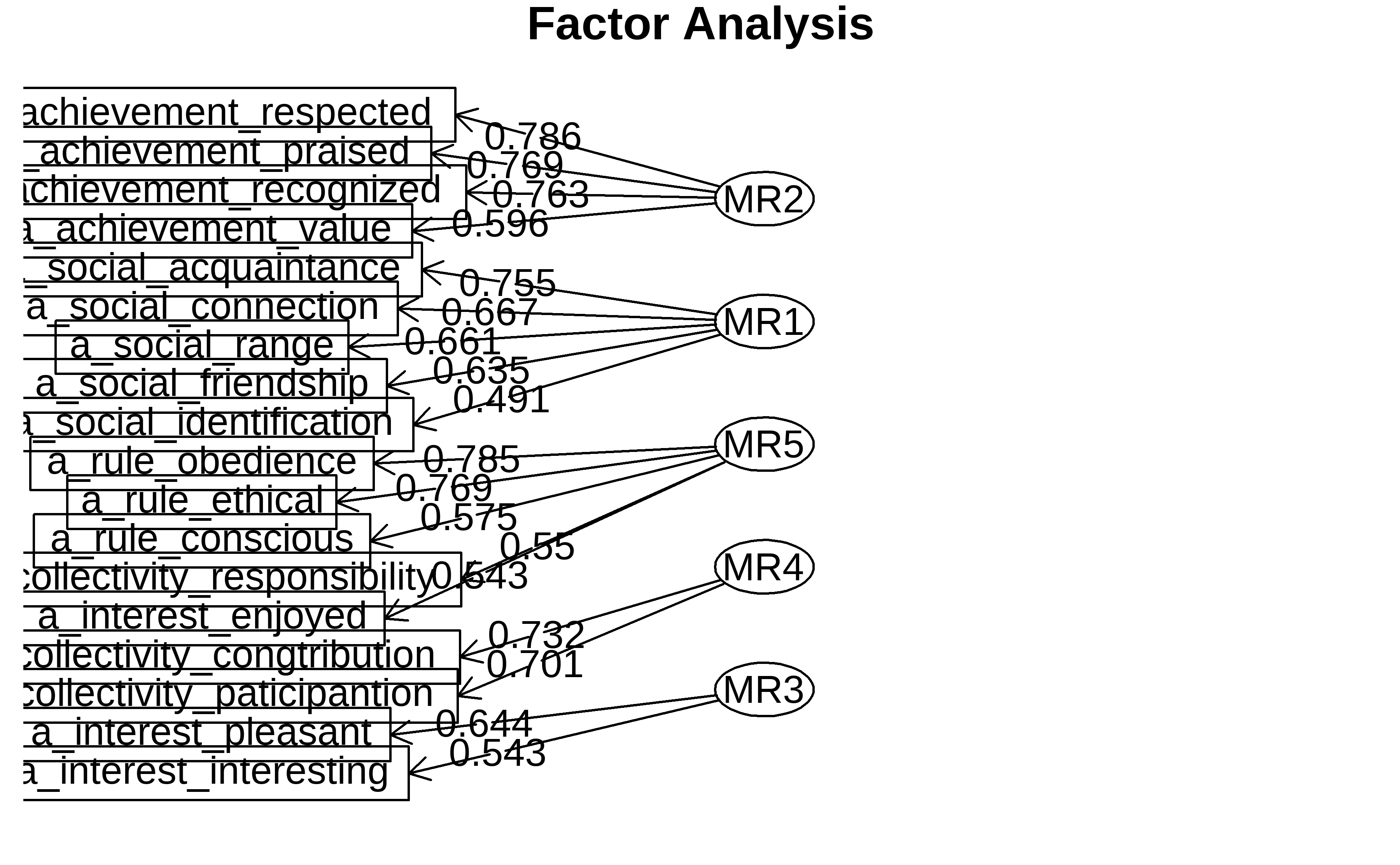
Figure 4.8: Loadings of EFA on the Employee’s Motivation for Knowledge Sharing
Figure 4.8 depicts the correspondence between the 5 common factors and the 18 original variables. In particular, the items of a_achievement_recognized, a_achievement_praised, a_achievement_respected and a_achievement_value(Q1-Q4) have high loadings on Factor1, which mainly reflects the employee’s perception of achievement. The items of a_social_identification, a_social_range, a_social_acquaintance, a_social_friendship, and a_social_connection(Q8-Q12) have high loadings on Factor2, which mainly reflects the employee’s construction of social relations. Notably, Factor1 and Factor2 are the same in the two dimensions of the employee’s motivation for knowledge scale. The items of a_rule_obedience, a_rule_ethical, a_rule_conscious, a_collectivity_responsibility, and a_interest_enjoyed(Q16-Q18, Q7, and Q15) have high loadings on Factor3. The items of a_collectivity_congtribution and a_collectivity_paticipantion(Q5-Q6) have high loadings on Factor4. The items of a_interest_interesting and a_interest_pleasant(Q13-Q14) have high loadings on Factor5. While the latter three factors are a little different from the dimensions division of the employee’s motivation for knowledge sharing scale. The author renamed them Individual and Collective Consciousness, Collective Behaviors, and Personal Preference, respectively.
- Table 4.19: New Independent Variables and Factor Scores
df_new <- as_tibble(Mod1$scores) %>%
  bind_cols(df) %>%
  relocate(id, .before = MR2) %>%
  rename(
    "Perception_of_Achievement" = MR2,
    "Construction_of_Social_Relations" = MR1,
    "Individual_and_Collective_Consciousness" = MR5,
    "Collective_Behaviors" = MR4,
    "Personal_Preference" = MR3
  )
as_tibble(Mod1$scores) %>% head() %>% knitr::kable(caption = "New Independent Variables and Factor Scores")| MR2 | MR1 | MR5 | MR4 | MR3 |
|---|---|---|---|---|
| -2.250 | -0.112 | -0.904 | 1.687 | -3.299 |
| -0.327 | -0.464 | 0.157 | -0.273 | -0.137 |
| -0.327 | -0.464 | 0.157 | -0.273 | -0.137 |
| -0.274 | 0.251 | -0.904 | -2.730 | -0.916 |
| -0.327 | -0.464 | 0.157 | -0.273 | -0.137 |
| -0.235 | 0.623 | -2.155 | 0.515 | 2.279 |
Table 4.19 shows the result of factor scores. Next, these five new variables will be considered as the new independent variables in a linear regression analysis with the dependent variable, employee creativity.
4.3.5 Linear regression analysis
df_regress <- df_new %>%
  rowwise() %>%
  mutate(Creativity = mean(c_across(cols = starts_with("b_")))) %>%
  ungroup() %>%
  mutate( across(gender:position_level, as.factor) ) %>%
relocate(Creativity, .after = id)- Mod2: The linear model of the control variables and the dependent variable, see Equation (4.2)
\[\begin{align*} \operatorname{Creativity} = \alpha + \beta_{1}(\operatorname{gender}_{\operatorname{1}}) + \beta_{2}(\operatorname{age}_{\operatorname{2}}) + \beta_{3}(\operatorname{age}_{\operatorname{4}}) + \beta_{4}(\operatorname{age}_{\operatorname{1}}) + \beta_{5}(\operatorname{educational\_background}_{\operatorname{2}}) + \beta_{6}(\operatorname{educational\_background}_{\operatorname{3}}) + \beta_{7}(\operatorname{educational\_background}_{\operatorname{1}}) + \beta_{8}(\operatorname{work\_experience}_{\operatorname{2}}) + \beta_{9}(\operatorname{work\_experience}_{\operatorname{3}}) + \beta_{10}(\operatorname{work\_experience}_{\operatorname{1}}) + \beta_{11}(\operatorname{position\_level}_{\operatorname{2}}) + \beta_{12}(\operatorname{position\_level}_{\operatorname{3}}) + \beta_{13}(\operatorname{position\_level}_{\operatorname{4}}) + \epsilon \tag{4.2} \end{align*}\]
- Mod3: The linear model of the five new variables and the dependent variable, see Equation (4.3)
\[\begin{align*} \operatorname{Creativity} = \alpha + \beta_{1}(\operatorname{gender}_{\operatorname{1}}) + \beta_{2}(\operatorname{age}_{\operatorname{2}}) + \beta_{3}(\operatorname{age}_{\operatorname{4}}) + \beta_{4}(\operatorname{age}_{\operatorname{1}}) + \beta_{5}(\operatorname{educational\_background}_{\operatorname{2}}) + \beta_{6}(\operatorname{educational\_background}_{\operatorname{3}}) + \beta_{7}(\operatorname{educational\_background}_{\operatorname{1}}) + \beta_{8}(\operatorname{work\_experience}_{\operatorname{2}}) + \beta_{9}(\operatorname{work\_experience}_{\operatorname{3}}) + \beta_{10}(\operatorname{work\_experience}_{\operatorname{1}}) + \beta_{11}(\operatorname{position\_level}_{\operatorname{2}}) + \beta_{12}(\operatorname{position\_level}_{\operatorname{3}}) + \beta_{13}(\operatorname{position\_level}_{\operatorname{4}}) + \beta_{14}(\operatorname{Perception\_of\_Achievement}) + \beta_{15}(\operatorname{Construction\_of\_Social\_Relations}) + \beta_{16}(\operatorname{Individual\_and\_Collective\_Consciousness}) + \beta_{17}(\operatorname{Collective\_Behaviors}) + \beta_{18}(\operatorname{Personal\_Preference}) + \epsilon \tag{4.3} \end{align*}\]
Two linear regression models are proposed to test Hypothesis 3: the Mod2, employee creativity as the dependent variable, only take the gender, age, educational background, work experience, and position level as the control variables, see Equation (4.2). Then, adding the new five variables, i.e., Perception of Achievement, Construction of Social Relations, Individual and Collective Consciousness, Collective Behaviors, and Personal Preference, into Mod2 as the independent variables, see Equation (4.3).
- Table 4.20: The Results of Linear Regression Analysis
Table4_Mod2 <- Mod2 %>% tbl_regression()
Table4_Mod3 <- Mod3 %>% tbl_regression()
tbl_merge(tbls = list(Table4_Mod2, Table4_Mod3)) %>%
modify_spanning_header(everything() ~ "The Results of Linear Regression Analysis") %>% modify_caption("The Results of Linear Regression Analysis")| The Results of Linear Regression Analysis | ||||||
|---|---|---|---|---|---|---|
| Characteristic | Beta | 95% CI1 | p-value | Beta | 95% CI1 | p-value |
| gender | ||||||
| 1 | — | — | — | — | ||
| 2 | -0.15 | -0.30, 0.01 | 0.062 | 0.01 | -0.07, 0.09 | 0.9 |
| age | ||||||
| 1 | — | — | — | — | ||
| 2 | -0.27 | -0.51, -0.03 | 0.029 | -0.14 | -0.27, -0.02 | 0.021 |
| 3 | -0.15 | -0.39, 0.09 | 0.2 | -0.11 | -0.23, 0.01 | 0.078 |
| 4 | -0.05 | -0.31, 0.21 | 0.7 | -0.16 | -0.29, -0.03 | 0.017 |
| educational_background | ||||||
| 1 | — | — | — | — | ||
| 2 | -0.06 | -0.64, 0.53 | 0.9 | 0.04 | -0.26, 0.33 | 0.8 |
| 3 | -0.13 | -0.70, 0.45 | 0.7 | 0.03 | -0.26, 0.32 | 0.8 |
| 4 | -0.26 | -0.86, 0.35 | 0.4 | 0.02 | -0.29, 0.32 | >0.9 |
| work_experience | ||||||
| 1 | — | — | — | — | ||
| 2 | 0.05 | -0.18, 0.28 | 0.6 | 0.03 | -0.08, 0.15 | 0.6 |
| 3 | -0.07 | -0.30, 0.16 | 0.5 | -0.01 | -0.12, 0.11 | >0.9 |
| 4 | 0.12 | -0.14, 0.37 | 0.4 | 0.05 | -0.07, 0.18 | 0.4 |
| position_level | ||||||
| 1 | — | — | — | — | ||
| 2 | 0.13 | -0.11, 0.36 | 0.3 | 0.04 | -0.08, 0.16 | 0.5 |
| 3 | 0.22 | -0.08, 0.52 | 0.2 | -0.02 | -0.17, 0.13 | 0.8 |
| 4 | 0.15 | -0.17, 0.47 | 0.4 | -0.23 | -0.40, -0.06 | 0.007 |
| Perception_of_Achievement | 0.25 | 0.21, 0.29 | <0.001 | |||
| Construction_of_Social_Relations | 0.35 | 0.31, 0.39 | <0.001 | |||
| Individual_and_Collective_Consciousness | 0.35 | 0.31, 0.39 | <0.001 | |||
| Collective_Behaviors | 0.26 | 0.21, 0.30 | <0.001 | |||
| Personal_Preference | 0.28 | 0.23, 0.32 | <0.001 | |||
| 1 CI = Confidence Interval | ||||||
- Figure 4.9: Combination of Modeling and Statistics
ggcoefstats(Mod3, output = "plot")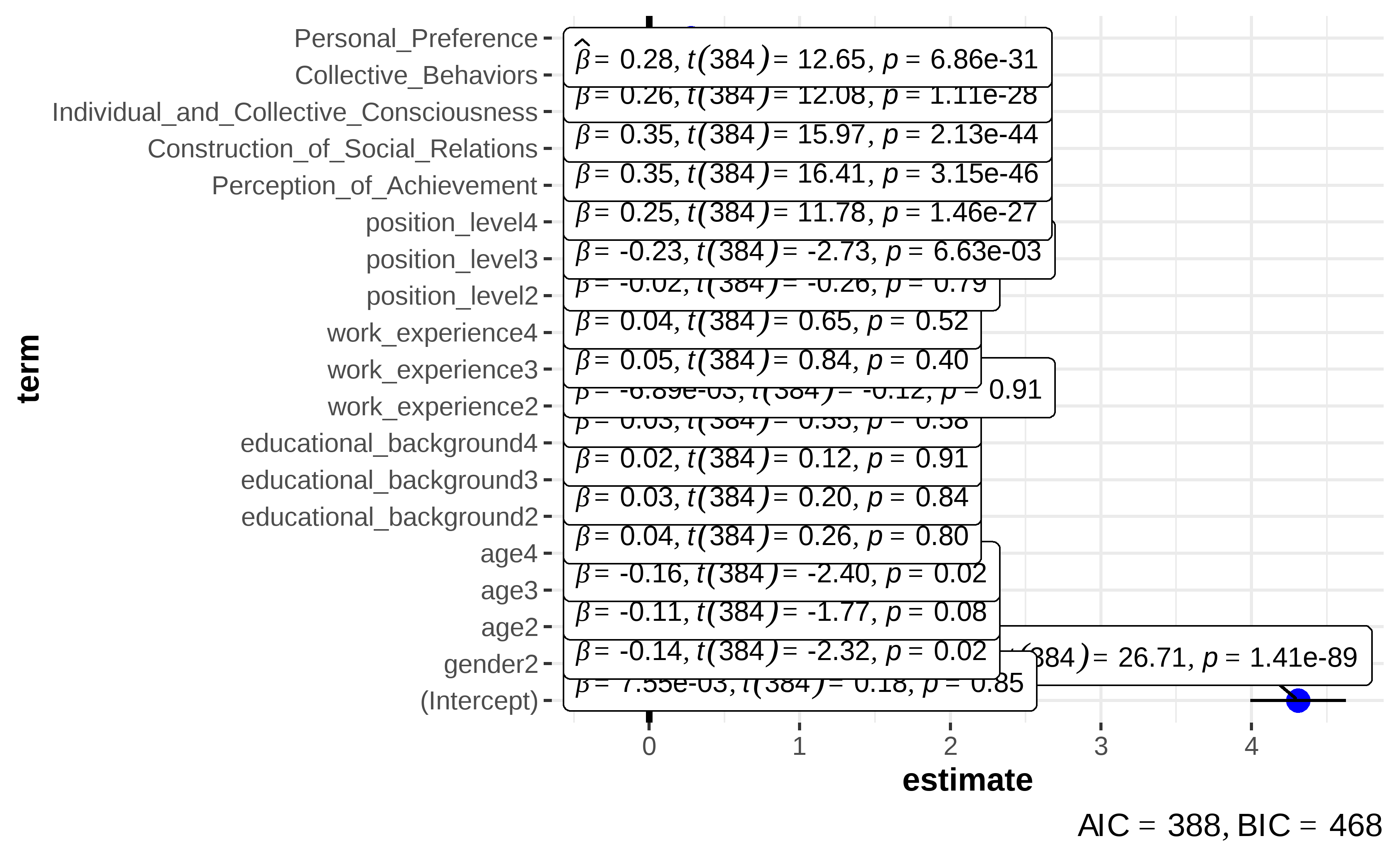
Figure 4.9: Combination of Modeling and Statistics
According to the results show in Table 4.20, we can infer that Mod2 explains a statistically not significant and weak proportion of variance, as R^2 = 0.05. Conversely, Mod3 explains a statistically significant and substantial proportion of variance, as R^2 = 0.76. Meanwhile, the effect of Perception of Achievement(Mod3, β = 0.251713, p < 2e-16), Construction of Social Relations(Mod3, β = 0.346645, p < 2e-16), Individual and Collective Consciousness(Mod3, β = 0.349288, p < 2e-16), Collective Behaviors(Mod3, β = 0.256346, p < 2e-16) and Personal Preference(Mod3, β = 0.277235, p < 2e-16) are all statistically significant and positive. Thus, Hypothesis 3 is supported.
- Figure 4.10: The tendencies and predictions
p1 <- marginaleffects::plot_cap(Mod3, condition = "Perception_of_Achievement")
p2 <- marginaleffects::plot_cap(Mod3, condition = "Construction_of_Social_Relations")
p3 <- marginaleffects::plot_cap(Mod3, condition = "Individual_and_Collective_Consciousness")
p4 <- marginaleffects::plot_cap(Mod3, condition = "Collective_Behaviors")
p5 <- marginaleffects::plot_cap(Mod3, condition = "Personal_Preference")

(p1 + p2 + p3 + p4 + p5) +
  plot_layout(guides = "collect") +
  plot_annotation(
    title = "The Tendencies on five common factors of the Employee's Motivation for Knowledge Sharing and Employee Creativity",
    theme = theme(
      plot.title = element_text(size = rel(0.6), face = "bold"),
      legend.position = "bottom"
    )
  ) +
  theme_clean()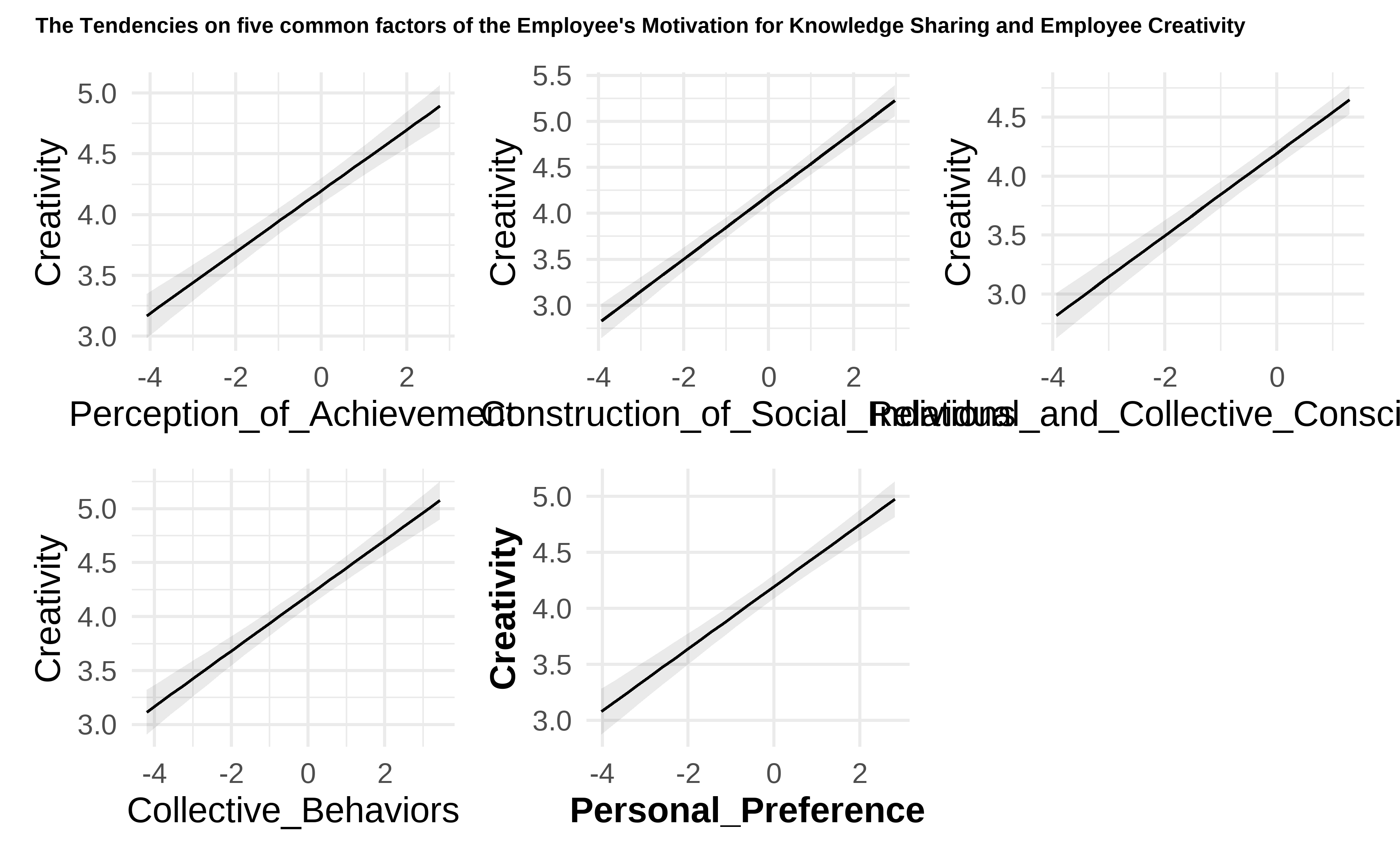
Figure 4.10: The tendencies and predictions
Figure 4.10 shows the tendencies in five common factors of the Employee’s Motivation for Knowledge Sharing and Employee Creativity. This figure depicts the prediction of employee creativity against the values of five predictors, respectively. It indicates a positive proportional relationship between all the five common factors of the employee’s motivation for knowledge sharing and employee creativity. It also provides a supporting basis for the conclusions of this study.