4 tmap4

This chapter explores some features of tmap4 such as visual variables and using a basemap.

Note that there are many basemaps served you might explore at https://leaflet-extras.github.io/leaflet-providers/preview/index.html. However, not all are supported by tm_basemap, so they may end up blank. Unfortunately, the various USGS basemaps are currently not supported, but the Esri and Open basemaps are generally reliable.

4.1 Simple test

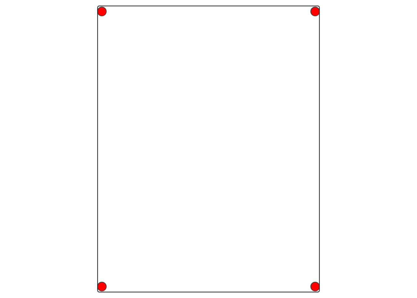
We’ll start with a simple test of tmap on a basemap, with coordinates of 4 points in the NW part of Lake Tahoe provided in code.

library(tmap)
tmap_mode("plot")
loc = c("nw","ne","sw","se")
lon = c(-120.25, -120.0, -120.25, -120.0)
lat = c(39.25, 39.25, 39.0, 39.0)
df = data.frame(loc,lon,lat)
tahoeNW <- sf::st_as_sf(df, coords = c("lon","lat"), crs=4326)
tm_basemap("Esri.WorldTopoMap") + # USGS.USTopo") + # 
  tm_graticules() +
  tm_shape(tahoeNW) + tm_dots()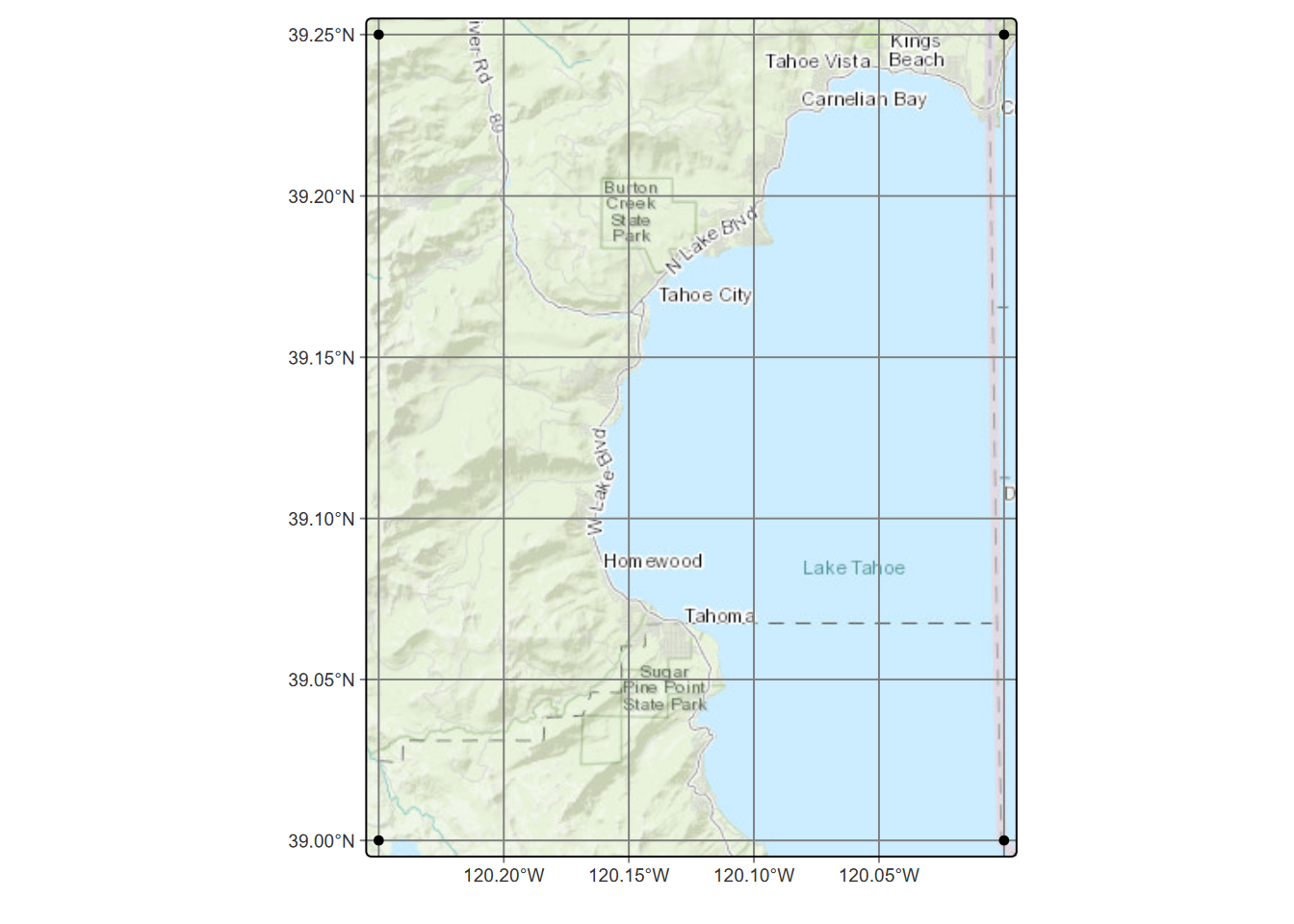

Now we’ll add symbology to the points, sticking with simple tm_dots.

library(tmap)
tmap_mode("plot")
loc = c("nw","ne","sw","se")
lon = c(-120.25, -120.0, -120.25, -120.0)
lat = c(39.25, 39.25, 39.0, 39.0)
df = data.frame(loc,lon,lat)
tahoeNW <- sf::st_as_sf(df, coords = c("lon","lat"), crs=4326)
tm_basemap("Esri.WorldTopoMap") +
  tm_graticules() +
  tm_shape(tahoeNW) + tm_dots(fill="red", size=0.7)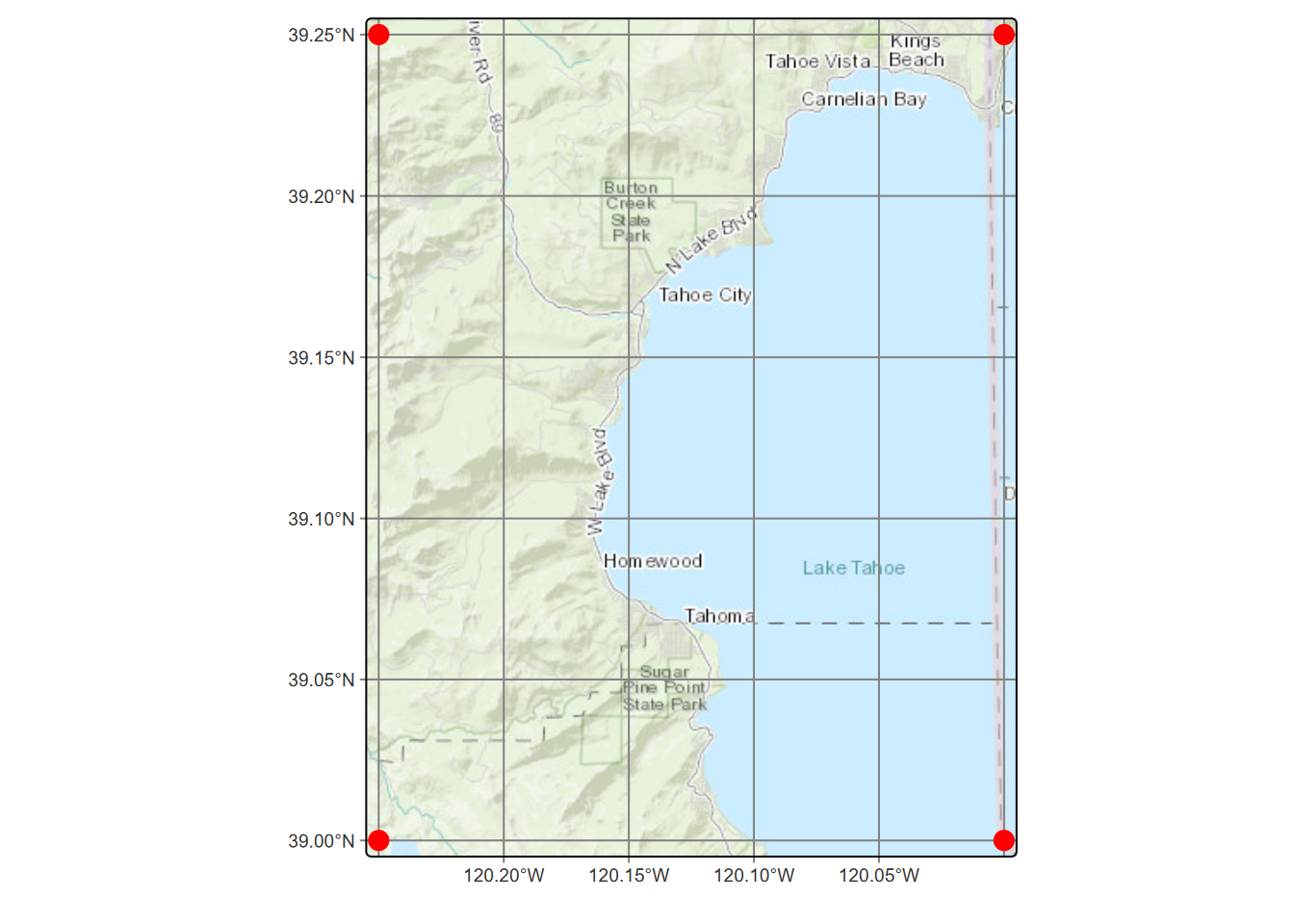

Now we’ll specify a particular point symbol, using the R shape 21 for a filled circle (google R point symbols to see the 25 shapes).

library(tmap)
tmap_mode("plot")
loc = c("nw","ne","sw","se")
lon = c(-120.25, -120.0, -120.25, -120.0)
lat = c(39.25, 39.25, 39.0, 39.0)
df = data.frame(loc,lon,lat)
tahoeNW <- sf::st_as_sf(df, coords = c("lon","lat"), crs=4326)
tm_basemap("Esri.WorldTopoMap") +
  tm_graticules() +
  tm_shape(tahoeNW) + tm_symbols(shape=21, fill="red", size=0.7, col="black")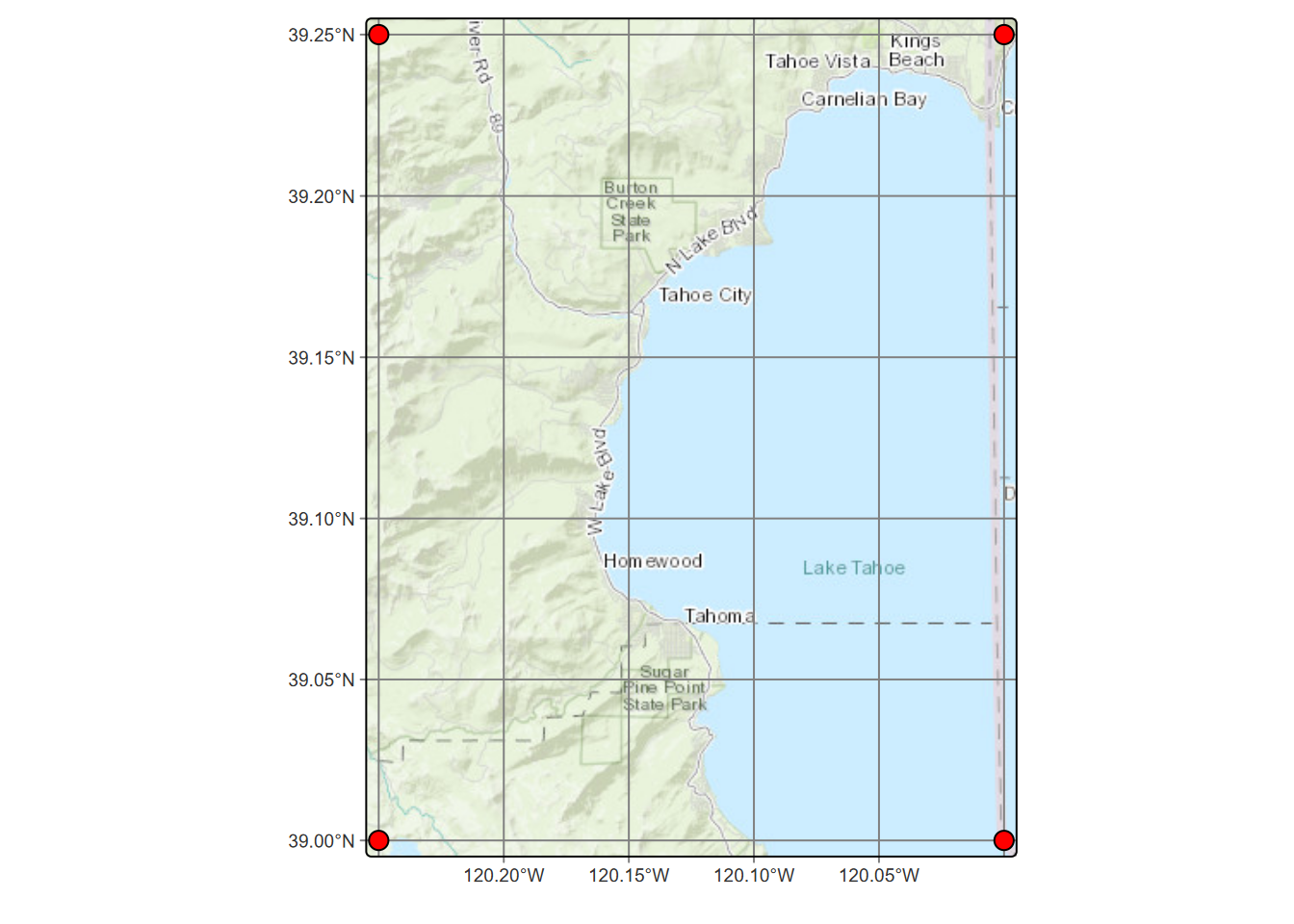

4.2 Visual variables

There are two kinds of variables that tmap4 responds to – transformation variables that changes the display spatial coordinates (such as in a cartogram) and visual variables that change the symbology. Visual variables will be most useful for us, so is the main subject of this chapter.

From a vignette by Martijn Tennekes, we can see the a table of visual variables supported:

Map layer	Visual variables	Visual constant
`tm_basemap()`	none	`alpha`
`tm_polygons()`	`fill` (fill color), `col` (border color), `lwd` (border line width) `lty` (border line type), `fill_alpha` (fill transparency), `col_alpha` (border color transparency)	`linejoin` (line join) and `lineend` (line end)
`tm_symbols()`	`fill` (fill color), `col` (border color), `size`, `shape`, `lwd` (border line width) `lty` (border line type), `fill_alpha` fill transparency, `col_alpha` border color transparency	`linejoin` (line join) and `lineend` (line end)
`tm_lines()`	`col` (color), `lwd` (line width) `lty` (line type), `alpha` transparency	`linejoin` (line join) and `lineend` (line end)
`tm_raster()`	`col` (color), `alpha` (transparency)
`tm_text()`	`size`, `col`

4.3 Constant visual variables

tm_shape(tahoeNW) + tm_symbols(size=1, fill="red")

tm_shape(World) + tm_polygons("gray")

## Using a visual variable for feature symbolization

tm_shape(World) +
  tm_polygons("pop_est")

You can create facets by specifying multiple data variable names and scales to one visual (or transformation) variable, in this case "fill". The effect will be a comparison of six symbolization methods using the same variable.

data(World)
Africa = World[World$continent == "Africa", ]
Africa$life_exp = round(Africa$life_exp)
tm_shape(Africa) +
    tm_polygons(rep("life_exp", 6), 
                fill.scale = list(tm_scale_categorical(),
                                  tm_scale_ordinal(),
                                  tm_scale_intervals(),
                                  tm_scale_continuous(),
                                  tm_scale_continuous_log(),
                                  tm_scale_discrete()),
                fill.legend = tm_legend(title = "", position = tm_pos_in("left", "top"))) +
    tm_layout(panel.labels = c("tm_scale_categorical", "tm_scale_ordinal", "tm_scale_intervals", "tm_scale_continuous", "tm_scale_continuous_log", "tm_scale_discrete"), 
              inner.margins = c(0.05, 0.4, 0.1, 0.05),
              legend.text.size = 0.5)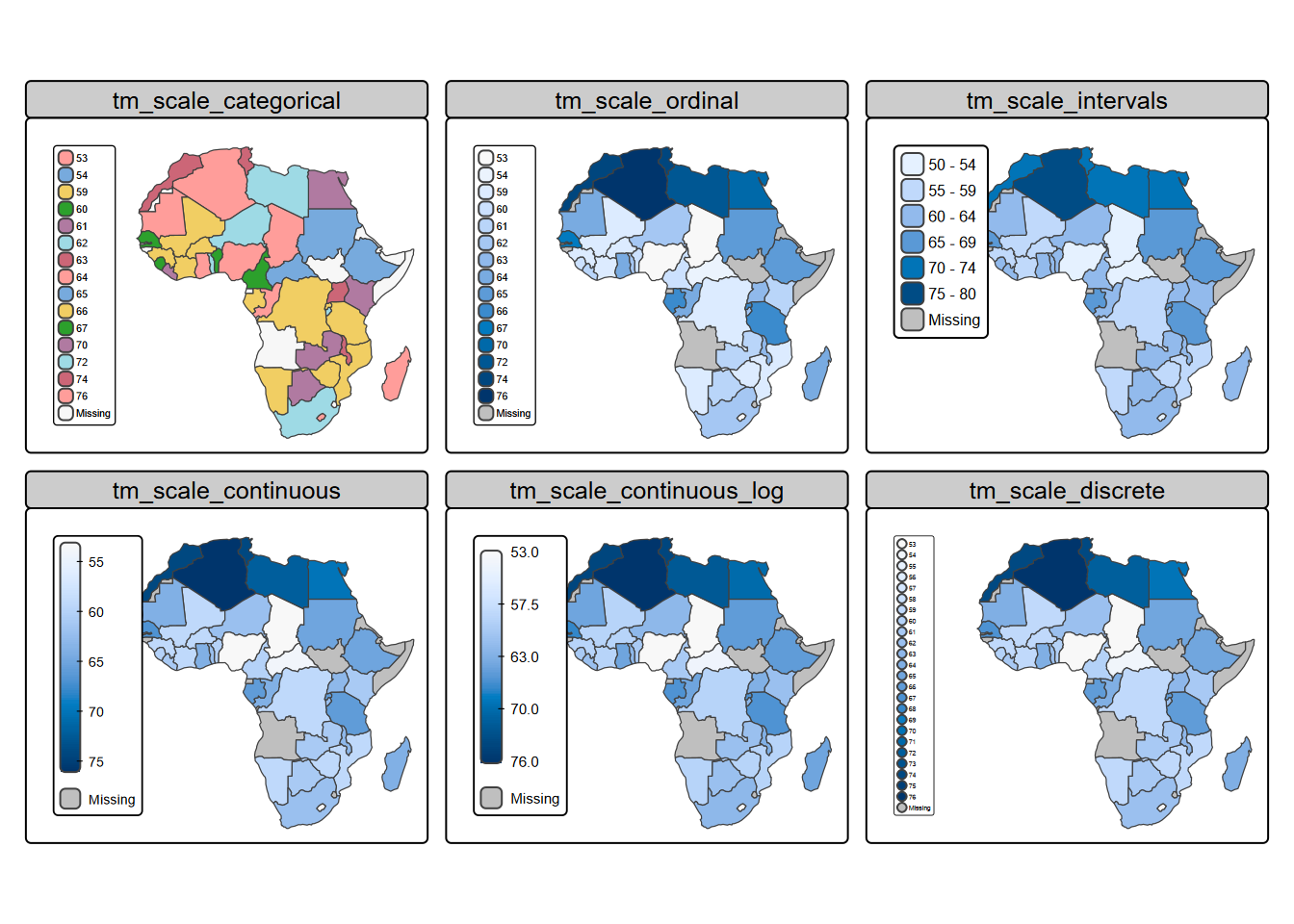

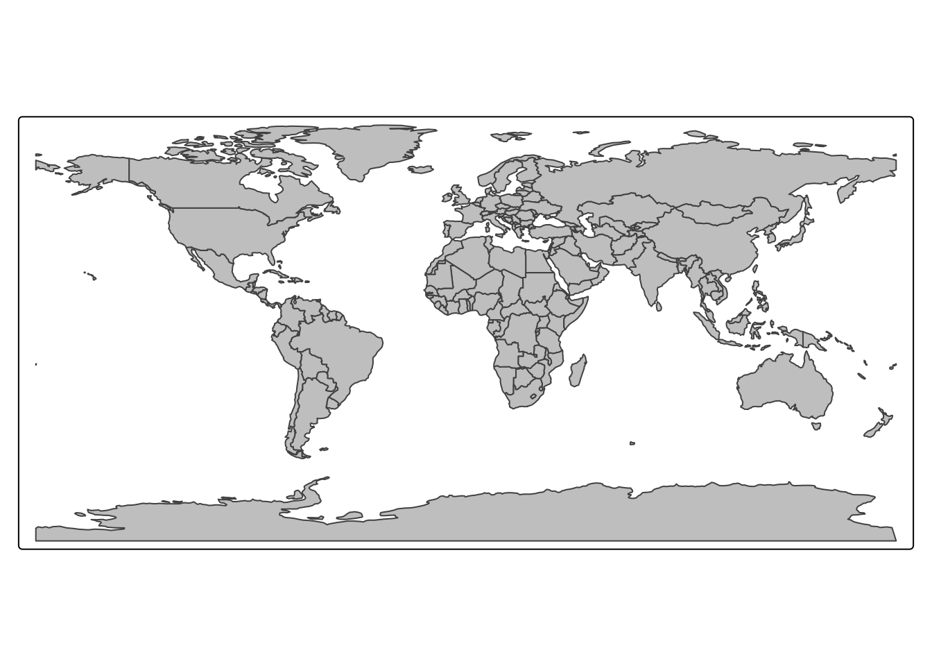
4.4 Basemap

Basemaps are very useful for providing context for thematic maps. The tm_basemap function in tmap uses a capability of leaflet interactive maps for this, and makes use of the maptiles package to provide this capability for static (plot mode) maps.

tm_basemap(server="OpenTopoMap", zoom=2) +
  tm_shape(World, bbox=sf::st_bbox(c(xmin=-180,xmax=180,ymin=-85,ymax=85))) +
  tm_polygons(fill=NA,col="black") +
  tm_layout(inner.margins=rep(0,4))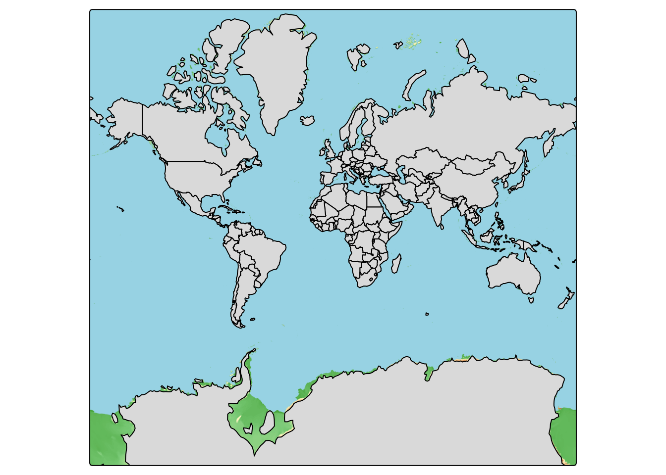

4.4.1 Basemaps with rasters

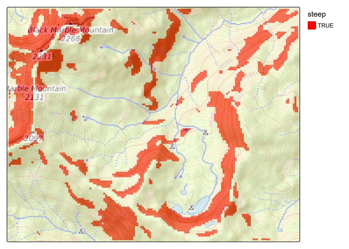
The tm_basemap method in the current tmap 4.0 version works fine with feature data, but to get a basemap when you want to display rasters as well requires another method, using maptiles::get_tiles and displaying that as a raster. To display rasters together requires an alpha setting, so we’ll use that with the basemap since it will need to go on top to scale correctly.

library(terra); library(igisci); library(maptiles); library(tmap)
elev <- rast(ex("marbles/elev.tif"))
slope <- terrain(elev, v="slope")
steep <- slope > 30
steep[steep==0] <- NA
mblBase <- get_tiles(steep, provider="OpenTopoMap")
tm_shape(steep) + 
  tm_raster(col.scale=tm_scale_categorical(values=c("red")),
            col.legend = tm_legend("steep", frame=F)) +
  tm_shape(mblBase) + 
     tm_rgb(col_alpha=0.5)