1 Background, Goals and Data

The purpose of this bookdown book is to provide Addenda to Introduction to Environmental Data Science, at https://bookdown.org/igisc/EnvDataSci/ to include case studies, extended and experimental methods, and guides for building packages and RMarkdown documents. It’ll serve as a sandbox for exploring methods, some of which will make it into the Introduction to Environmental Data Science book.

1.1 Structure of the Addenda

These addenda may include:

Case studies and extended methods, such as
- air pollution studies
- mapping methods
- exploring other interpolation methods
- models, e.g. a more extended seabird model
- meadow research we’re doing, in time and space domains
- other imagery classification methods
Guides
- RMarkdown
- Building code and data packages on GitHub

See specifics in the table of contents.

Note: some of these methods have made it into the main book, possibly in reduced form. The intention is in part to allow for a more extensive treatment in this addenda, and for the clearest and most succinct examples to make it to the next edition of the book, possibly replacing methods that might be moved here, as useful though not essential. And that’s a good example of a non-succinct sentence, so it belongs here…

1.2 Software and Data

Some things covered in the main book, but repeated here for convenience.

## [1] "This book was produced in RStudio using R version 4.3.1 (2023-06-16 ucrt)"

For a start, you’ll need to have R and RStudio installed, then you’ll need to install various packages to support specific chapters and sections. No instructions are provided here, since you should know how to install packages in RStudio.

From time to time, you’ll want to update your installed packages, and that usually happens when something doesn’t work and maybe the dependencies of one package on another gets broken with a change in a package. Fortunately, in the R world, especially at the main repository at CRAN, there’s a lot of effort put into making sure packages work together, so usually there are no surprises if you’re using the most current versions.

Once a package like dplyr is installed, you can access all of its functions and data by adding a library call, like …

library(dplyr)

… which you will want to include in your code, or to provide access to multiple libraries in the tidyverse, you can use library(tidyverse). Alternatively, if you’re only using maybe one function out of an installed package, you can call that function with the :: separator, like dplyr::select(). This method has another advantage in avoiding problems with duplicate names – and for instance we’ll generally call dplyr::select() this way.

1.2.1 Data

We’ll be using data from various sources, including data on CRAN like the code packages above which you install the same way – so use install.packages("palmerpenguins").

We’ve also created a repository on GitHub that includes data we’ve developed in the Institute for Geographic Information Science (iGISc) at SFSU, and you’ll need to install that package a slightly different way.

GitHub packages require a bit more work on the user’s part since we need to first install remotes¹, then use that to install the GitHub data package:

install.packages("remotes")
remotes::install_github("iGISc/igisci")

Then you can access it just like other built-in data by including:

library(igisci)

To see what’s in it, you’ll see the various datasets listed in:

data(package="igisci")

For instance, Figure 1.1 is a map of California counties using the CA_counties sf feature data. We’ll be looking at the sf (Simple Features) package later in the Spatial section of the book, but seeing library(sf), this is one place where you’d need to have installed another package, with install.packages("sf").

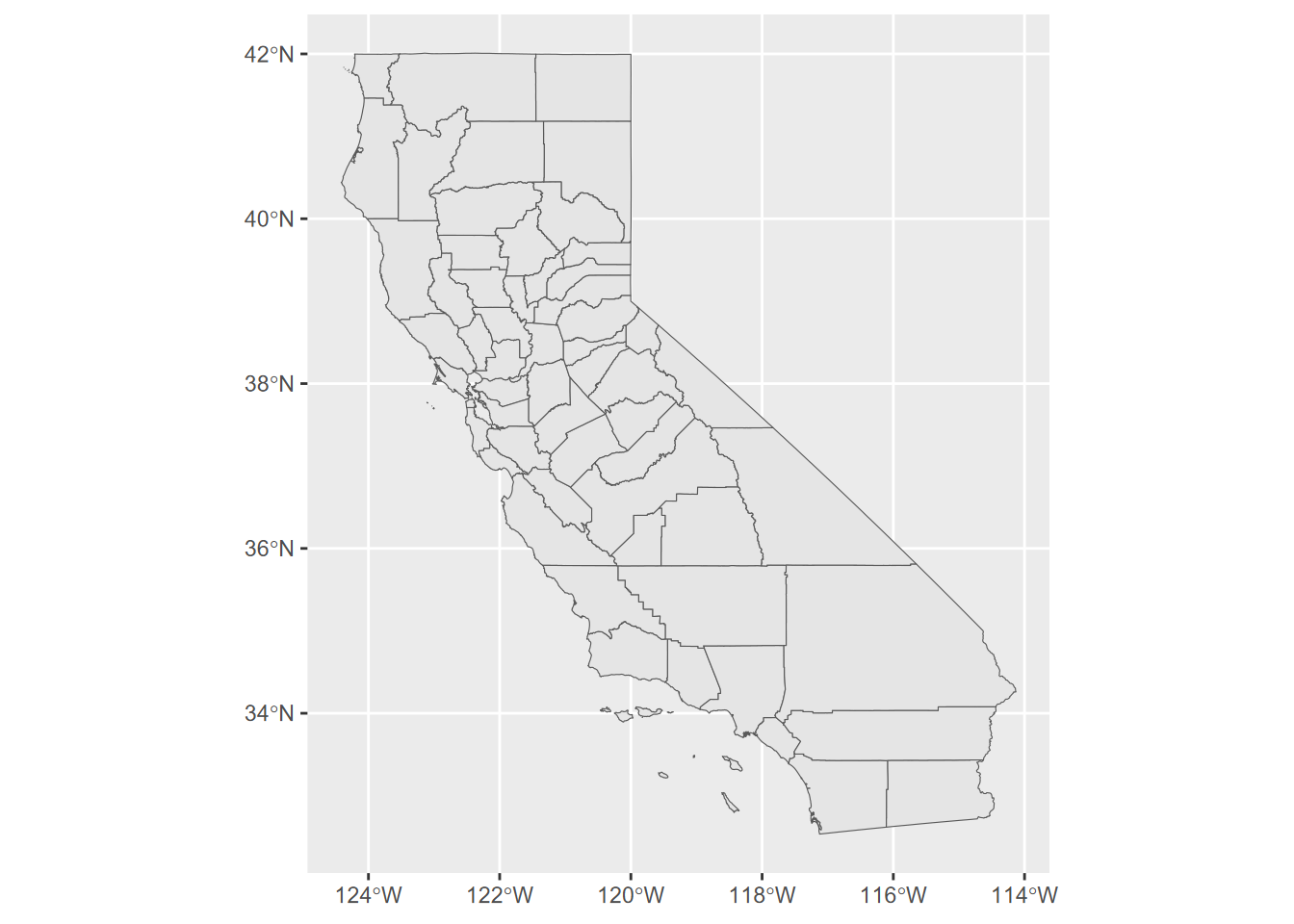
library(tidyverse); library(igisci); library(sf)
ggplot(data=CA_counties) + geom_sf()

FIGURE 1.1: California counties simple features data in igisci package

The package datasets can be used directly as sf data or data frames. And similarly to functions, you can access the (previously installed) data set by prefacing with igisci:: this way, without having to load the library. This might be useful in a one-off operation:

mean(igisci::sierraFeb$LATITUDE)

## [1] 38.3192

Raw data such as .csv files can also be read from the extdata folder that is installed on your computer when you install the package, using code such as:

csvPath <- system.file("extdata","TRI/TRI_1987_BaySites.csv", package="igisci")
TRI87 <- read_csv(csvPath)

or something similar for shapefiles, such as:

shpPath <- system.file("extdata","marbles/trails.shp", package="igisci")
trails <- st_read(shpPath)

And we’ll find that including most of the above arcanity in a function will help. We’ll look at functions later, but here’s a function that we’ll use a lot for setting up reading data from the extdata folder:

ex <- function(dta){system.file("extdata",dta,package="igisci")}

And this ex()function is needed so often that it’s installed in the igisci package, so if you have library(igisci) in effect, you can just use it like this:

trails <- st_read(ex("marbles/trails.shp"))

But how do we see what’s in the extdata folder? We can’t use the data() function, so we would have to dig for the folder where the igisci package gets installed, which is buried pretty deeply in your user profile. So I wrote another function exfiles() that creates a data frame showing all of the files and the paths to use. In RStudio you could access it with View(exfiles()) or we could use a datatable (you’ll need to have installed “DT”). You can use the path using the ex() function with any function that needs it to read data, like read.csv(ex('CA/CA_ClimateNormals.csv')), or just enter that ex() call in the console like ex('CA/CA_ClimateNormals.csv') to display where on your computer the installed data reside.

DT::datatable(exfiles(), options=list(scrollX=T), rownames=F)

1.3 Acknowledgements

This compilation includes data and methods gathered by students in San Francisco State’s GEOG 604/704 Environmental Data Science class, colleagues in the Department of Geography & Environment and NGOs such as PointBlue. And thanks again to Anna Studwell for the nice cover art: “Dandelion fluff – Ephemeral stalk sheds seeds to the universe”.

Note: you can also use devtools instead of remotes if you have that installed. They do the same thing; remotes is a subset of devtools. If you see a message about Rtools, you can ignore it since that is only needed for building tools from C++ and things like that.↩︎

Environmental Data Science Addenda