9 Curve fitting, with examples from Red Clover Valley carbon flux and gullies

This section will explore various curve fitting methods, starting with some carbon flux tower data from Red Clover Valley. There’s not a lot of interpretation, as this is basically a sandbox for now…

9.1 Red Clover Valley flux data

Initial data read and time series charting

Some ideas for processing are from Mason Kealy. Data are from Andrew Oliphant.

9.1.1 Reading in the Excel File

First create a function to convert the first two rows into individual variables. We won’t include the units.

library(igisci); library(tidyverse); library(readxl)

read_excel2 <- function(xl){
  vnames <- read_excel(xl, n_max=0) |> names()
  vunits <- read_excel(xl, n_max=0, skip=1) |> names()
  read_excel(xl, skip=2, col_names=vnames)
}

In reading the data, we’ll remove the zero GPP_sum values.

Carbon_Flux <- read_excel2(ex("meadows/RCV_carbon_flux_data.xlsx")) |>
  filter(GPP_sum>0)

## New names:
## • `gCO2 m-2 d-1` -> `gCO2 m-2 d-1...2`
## • `gCO2 m-2 d-1` -> `gCO2 m-2 d-1...3`
## • `gCO2 m-2 d-1` -> `gCO2 m-2 d-1...4`
## • `degC` -> `degC...5`
## • `degC` -> `degC...6`
## • `degC` -> `degC...9`
## • `degC` -> `degC...10`
## • `degC` -> `degC...11`
## • `degC` -> `degC...12`
## • `0-1` -> `0-1...13`
## • `0-1` -> `0-1...14`
## • `0-1` -> `0-1...15`
## • `0-1` -> `0-1...16`

Mountflux <- Carbon_Flux %>% 
mutate_all(as.numeric) %>% 
mutate(DOY = as.Date(Date,format = "%m-%d")) %>% 
select(Date:PAR_ave) %>% 
mutate(NEE = round(NEE_sum, digits = 3), 
       GPP = round(GPP_sum, digits = 3),
       RE = round(RE_sum, digits = 3)) %>%
#select(-NEE_sum, -GPP_sum, -RE_sum) %>% 
  pivot_longer(cols = c("NEE", "RE", "GPP"), names_to = "CO2_FLUX_COMPONENTS", values_to ="value") %>%
  filter(GPP_sum != 0, !is.na(PAR_ave))

print(Mountflux)

## # A tibble: 906 × 9
##     Date GPP_sum NEE_sum RE_sum Tair_min Tair_max PAR_ave CO2_FLUX_COMPONENTS
##    <dbl>   <dbl>   <dbl>  <dbl>    <dbl>    <dbl>   <dbl> <chr>              
##  1    61   0.215    3.74   3.96    -8.32    13.0     420. NEE                
##  2    61   0.215    3.74   3.96    -8.32    13.0     420. RE                 
##  3    61   0.215    3.74   3.96    -8.32    13.0     420. GPP                
##  4    62   0.405    3.71   4.11    -6.75    14.8     424. NEE                
##  5    62   0.405    3.71   4.11    -6.75    14.8     424. RE                 
##  6    62   0.405    3.71   4.11    -6.75    14.8     424. GPP                
##  7    63   0.620    3.35   3.97    -7.84     9.47    480. NEE                
##  8    63   0.620    3.35   3.97    -7.84     9.47    480. RE                 
##  9    63   0.620    3.35   3.97    -7.84     9.47    480. GPP                
## 10    64   0.799    3.57   4.37    -4.99    11.8     474. NEE                
## # ℹ 896 more rows
## # ℹ 1 more variable: value <dbl>

9.1.2 Time series plot

Then I used ggplot to create a visualization of how NEE, GPP, an RE changed over a yearly time scale.

Mountflux %>% 
 ggplot(aes(x = Date, y= value, color = CO2_FLUX_COMPONENTS))+
  geom_line()+
  geom_hline(yintercept = 0, linetype = "longdash", color = "black")+
  ggtitle(" Red Clover Valley: Interannual Components of Carbon Flux Measurements") +
  xlab("Day of Year") +
  ylab("g C/m^2")+
  labs(caption =
"Figure 1: Components of Carbon Flux measurements collected in 30 minute intervals in 2021
and added into ‘sum daily value’ , from flux tower in Red Clover Valley,California. Components included NEE (Net Ecosystem Exchange), RE (Respiration Efficiency), GPP (Gross Primary Productivity) all measured in g C m^2 and are plotted against an annual time scale with days as the unit of measure.")

9.1.3 Pairs plot

Carbon_Flux |>
  select(GPP_sum:vpd_max) |>
  GGally::ggpairs()

  # pairs()

9.1.4 Non-linear model of PAR_ave ~ GPP_sum, using Michaelis-Menten model

Not the right goal for a model between these variables, since GPP should derive from PAR, not the other way around. But it does illustrate asymptotic data.

First the scatter plot:

plot(Carbon_Flux$GPP_sum, Carbon_Flux$PAR_ave,xlab="GPP_sum", ylab="PAR_ave")

9.1.5 Try fitting a non-linear model (SSmicmen from base R)

Based on https://www.datacamp.com/tutorial/introduction-to-non-linear-model-and-insights-using-r

Using start values for Vm and K based on interpreting the graph. We’ll use nonlinear least squares (nls) and starting values of the two coefficients.

micmenMod <- nls(PAR_ave~(Vm)*GPP_sum/(K+GPP_sum), data=Mountflux, start=list(Vm=750,K=1))
summary(micmenMod)

## 
## Formula: PAR_ave ~ (Vm) * GPP_sum/(K + GPP_sum)
## 
## Parameters:
##    Estimate Std. Error t value Pr(>|t|)    
## Vm 819.0045    13.4911   60.71   <2e-16 ***
## K    5.0071     0.2573   19.46   <2e-16 ***
## ---
## Signif. codes:  0 '***' 0.001 '**' 0.01 '*' 0.05 '.' 0.1 ' ' 1
## 
## Residual standard error: 121.1 on 904 degrees of freedom
## 
## Number of iterations to convergence: 7 
## Achieved convergence tolerance: 8.843e-06

Calculate residual error

sse <- micmenMod$m$deviance()
null <- lm(PAR_ave~1, data=Mountflux)
sst <- data.frame(summary.aov(null)[[1]])$Sum.Sq
percent_variation_explained <- 100*(sst-sse)/sst
percent_variation_explained

## [1] 59.97658

plot(Mountflux$GPP_sum, Mountflux$PAR_ave,xlab="GPP_sum", ylab="PAR_ave")
 lines(Mountflux$GPP_sum, 
       predict(micmenMod,Mountflux),col=2)

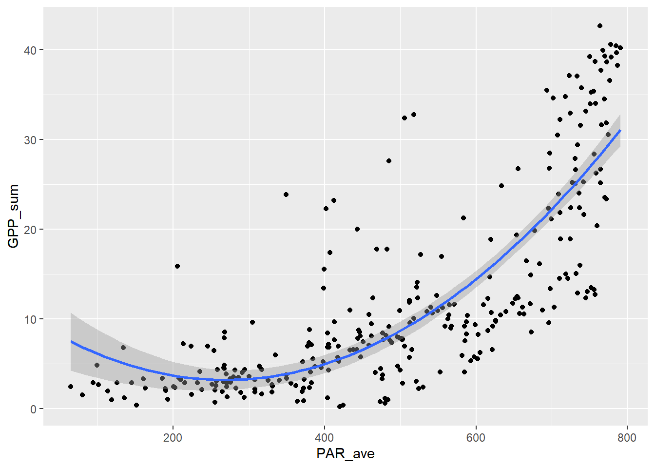
9.1.6 polynomial models

Ok, enough of that deceptive model of PAR predicted by GPP – not the way it works – and instead we’ll look at models that predict GPP from PAR, not asymptotic

plot(Mountflux$PAR_ave,Mountflux$GPP_sum, xlab="PAR_ave", ylab="GPP_sum")

9.1.6.1 poly 1

ord = 1
summary(lm(GPP_sum ~ poly(PAR_ave, ord, raw=T), data=Mountflux))

## 
## Call:
## lm(formula = GPP_sum ~ poly(PAR_ave, ord, raw = T), data = Mountflux)
## 
## Residuals:
##     Min      1Q  Median      3Q     Max 
## -11.944  -4.931  -1.131   4.287  19.711 
## 
## Coefficients:
##                              Estimate Std. Error t value Pr(>|t|)    
## (Intercept)                 -8.979814   0.669906  -13.40   <2e-16 ***
## poly(PAR_ave, ord, raw = T)  0.042818   0.001258   34.03   <2e-16 ***
## ---
## Signif. codes:  0 '***' 0.001 '**' 0.01 '*' 0.05 '.' 0.1 ' ' 1
## 
## Residual standard error: 7.242 on 904 degrees of freedom
## Multiple R-squared:  0.5616, Adjusted R-squared:  0.5611 
## F-statistic:  1158 on 1 and 904 DF,  p-value: < 2.2e-16

ggplot(Mountflux, aes(PAR_ave, GPP_sum)) + geom_point() +
  stat_smooth(method=lm, formula=y~poly(x,ord,raw=T))

9.1.6.2 poly 2

ord = 2
summary(lm(GPP_sum ~ poly(PAR_ave, ord, raw=T), data=Mountflux))

## 
## Call:
## lm(formula = GPP_sum ~ poly(PAR_ave, ord, raw = T), data = Mountflux)
## 
## Residuals:
##      Min       1Q   Median       3Q      Max 
## -14.9170  -3.5363  -0.4922   2.4821  23.4111 
## 
## Coefficients:
##                                Estimate Std. Error t value Pr(>|t|)    
## (Intercept)                   1.062e+01  1.269e+00   8.368   <2e-16 ***
## poly(PAR_ave, ord, raw = T)1 -5.500e-02  5.737e-03  -9.587   <2e-16 ***
## poly(PAR_ave, ord, raw = T)2  1.023e-04  5.892e-06  17.367   <2e-16 ***
## ---
## Signif. codes:  0 '***' 0.001 '**' 0.01 '*' 0.05 '.' 0.1 ' ' 1
## 
## Residual standard error: 6.273 on 903 degrees of freedom
## Multiple R-squared:  0.6714, Adjusted R-squared:  0.6706 
## F-statistic: 922.3 on 2 and 903 DF,  p-value: < 2.2e-16

ggplot(Mountflux, aes(PAR_ave, GPP_sum)) + geom_point() +
  stat_smooth(method=lm, formula=y~poly(x,ord,raw=T))

9.1.6.3 poly 3

ord = 3
summary(lm(GPP_sum ~ poly(PAR_ave, ord, raw=T), data=Mountflux))

## 
## Call:
## lm(formula = GPP_sum ~ poly(PAR_ave, ord, raw = T), data = Mountflux)
## 
## Residuals:
##      Min       1Q   Median       3Q      Max 
## -16.4635  -3.3477  -0.8198   2.3854  24.5018 
## 
## Coefficients:
##                                Estimate Std. Error t value Pr(>|t|)    
## (Intercept)                  -7.290e+00  2.276e+00  -3.203  0.00141 ** 
## poly(PAR_ave, ord, raw = T)1  1.048e-01  1.804e-02   5.810 8.65e-09 ***
## poly(PAR_ave, ord, raw = T)2 -2.949e-04  4.309e-05  -6.845 1.41e-11 ***
## poly(PAR_ave, ord, raw = T)3  2.908e-07  3.127e-08   9.299  < 2e-16 ***
## ---
## Signif. codes:  0 '***' 0.001 '**' 0.01 '*' 0.05 '.' 0.1 ' ' 1
## 
## Residual standard error: 5.996 on 902 degrees of freedom
## Multiple R-squared:  0.7001, Adjusted R-squared:  0.6991 
## F-statistic: 701.9 on 3 and 902 DF,  p-value: < 2.2e-16

ggplot(Mountflux, aes(PAR_ave, GPP_sum)) + geom_point() +
  stat_smooth(method=lm, formula=y~poly(x,ord,raw=T))

9.1.6.4 poly 4

ord = 4
summary(lm(GPP_sum ~ poly(PAR_ave, ord, raw=T), data=Mountflux))

## 
## Call:
## lm(formula = GPP_sum ~ poly(PAR_ave, ord, raw = T), data = Mountflux)
## 
## Residuals:
##      Min       1Q   Median       3Q      Max 
## -17.0946  -2.9525  -0.7201   2.0130  23.8099 
## 
## Coefficients:
##                                Estimate Std. Error t value Pr(>|t|)    
## (Intercept)                   1.346e+01  3.769e+00   3.570 0.000375 ***
## poly(PAR_ave, ord, raw = T)1 -1.768e-01  4.493e-02  -3.936 8.93e-05 ***
## poly(PAR_ave, ord, raw = T)2  9.001e-04  1.804e-04   4.990 7.25e-07 ***
## poly(PAR_ave, ord, raw = T)3 -1.692e-06  2.927e-07  -5.782 1.02e-08 ***
## poly(PAR_ave, ord, raw = T)4  1.122e-09  1.647e-10   6.812 1.75e-11 ***
## ---
## Signif. codes:  0 '***' 0.001 '**' 0.01 '*' 0.05 '.' 0.1 ' ' 1
## 
## Residual standard error: 5.85 on 901 degrees of freedom
## Multiple R-squared:  0.7148, Adjusted R-squared:  0.7135 
## F-statistic: 564.5 on 4 and 901 DF,  p-value: < 2.2e-16

ggplot(Mountflux, aes(PAR_ave, GPP_sum)) + geom_point() +
  stat_smooth(method=lm, formula=y~poly(x,ord,raw=T))

9.1.6.5 poly 5

ord = 5
summary(lm(GPP_sum ~ poly(PAR_ave, ord, raw=T), data=Mountflux))

## 
## Call:
## lm(formula = GPP_sum ~ poly(PAR_ave, ord, raw = T), data = Mountflux)
## 
## Residuals:
##      Min       1Q   Median       3Q      Max 
## -17.0834  -2.7700  -0.7949   1.9559  23.4067 
## 
## Coefficients:
##                                Estimate Std. Error t value Pr(>|t|)  
## (Intercept)                   1.325e+00  6.746e+00   0.196   0.8443  
## poly(PAR_ave, ord, raw = T)1  4.446e-02  1.116e-01   0.398   0.6904  
## poly(PAR_ave, ord, raw = T)2 -4.500e-04  6.488e-04  -0.694   0.4881  
## poly(PAR_ave, ord, raw = T)3  1.931e-06  1.698e-06   1.137   0.2557  
## poly(PAR_ave, ord, raw = T)4 -3.295e-09  2.046e-09  -1.611   0.1076  
## poly(PAR_ave, ord, raw = T)5  1.999e-12  9.226e-13   2.166   0.0306 *
## ---
## Signif. codes:  0 '***' 0.001 '**' 0.01 '*' 0.05 '.' 0.1 ' ' 1
## 
## Residual standard error: 5.838 on 900 degrees of freedom
## Multiple R-squared:  0.7163, Adjusted R-squared:  0.7147 
## F-statistic: 454.4 on 5 and 900 DF,  p-value: < 2.2e-16

ggplot(Mountflux, aes(PAR_ave, GPP_sum)) + geom_point() +
  stat_smooth(method=lm, formula=y~poly(x,ord,raw=T))

9.1.7 power law relationship

powerModel <- lm(log(GPP_sum) ~ log(PAR_ave), data=Mountflux)
summary(powerModel)

## 
## Call:
## lm(formula = log(GPP_sum) ~ log(PAR_ave), data = Mountflux)
## 
## Residuals:
##     Min      1Q  Median      3Q     Max 
## -3.5030 -0.2995  0.0036  0.4460  1.8629 
## 
## Coefficients:
##              Estimate Std. Error t value Pr(>|t|)    
## (Intercept)   -7.0150     0.3034  -23.12   <2e-16 ***
## log(PAR_ave)   1.4869     0.0495   30.04   <2e-16 ***
## ---
## Signif. codes:  0 '***' 0.001 '**' 0.01 '*' 0.05 '.' 0.1 ' ' 1
## 
## Residual standard error: 0.7199 on 904 degrees of freedom
## Multiple R-squared:  0.4995, Adjusted R-squared:  0.499 
## F-statistic: 902.2 on 1 and 904 DF,  p-value: < 2.2e-16

ggplot(Mountflux, aes(log(PAR_ave), log(GPP_sum))) + geom_point() +
  stat_smooth(method=lm)

## `geom_smooth()` using formula = 'y ~ x'

Now plot without the log transformed axes, we’ll need to create the curve with the model, using the coefficients.

coeff = exp(powerModel$coefficients[1])
power = powerModel$coefficients[2]
fit_func <- function(x) coeff*x^power

fluxPlot <- ggplot(Mountflux) +
  geom_point(aes(x=PAR_ave,y=GPP_sum))
fluxPlot <- fluxPlot +
  stat_function(fun=fit_func, color="orange",lwd=2, alpha=0.5)
fluxPlot

fit_eq = paste("y = ", round(coeff,6), " x^", round(power,3))
fluxPlot <- fluxPlot +
  annotate("text",x=200,y=40,label=fit_eq,size=4)
fluxPlot

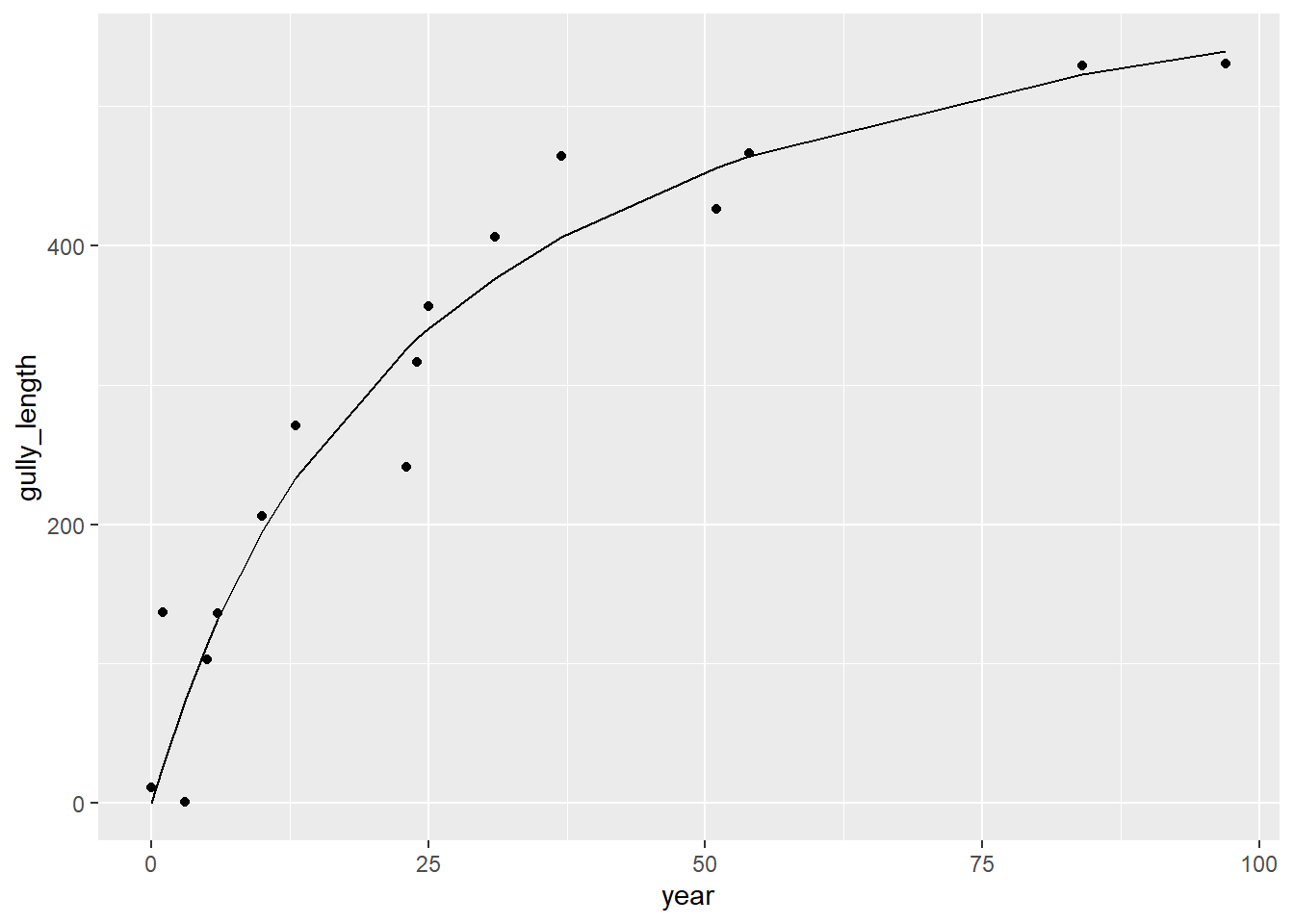
9.2 Another curve fit – of gullies that may follow a rate law of growth, or other asymptotic

from Graf WL (1977). The rate law in fluvial geomorphology. Am. J. Sci 277: 178-191.

The rate-law model that Graf used employs a half life, appropriate when depleting a quantity as will happen with an erosion phase following a disequilibrium (like a geomorphic drop in base level).

library(igisci); library(tidyverse)
gullyGrowth <- read_csv(ex("gully/gullyGrowth.csv"))

## Rows: 36 Columns: 3
## ── Column specification ────────────────────────────────────────────────────────
## Delimiter: ","
## chr (1): type
## dbl (2): distance, age_yrs
## 
## ℹ Use `spec()` to retrieve the full column specification for this data.
## ℹ Specify the column types or set `show_col_types = FALSE` to quiet this message.

ggplot(data=gullyGrowth, aes(x=distance, y=age_yrs, col=type)) +
  geom_point()

gully <- gullyGrowth |> filter(type=="gully")
gullyMod <- nls(age_yrs~(Vm)*distance/(K+distance), data=gully, start=list(Vm=1,K=1))
summary(gullyMod)

## 
## Formula: age_yrs ~ (Vm) * distance/(K + distance)
## 
## Parameters:
##    Estimate Std. Error t value Pr(>|t|)    
## Vm   86.156      4.733  18.204 4.86e-13 ***
## K   152.503     23.546   6.477 4.31e-06 ***
## ---
## Signif. codes:  0 '***' 0.001 '**' 0.01 '*' 0.05 '.' 0.1 ' ' 1
## 
## Residual standard error: 3.947 on 18 degrees of freedom
## 
## Number of iterations to convergence: 9 
## Achieved convergence tolerance: 8.225e-07

Calculate residual error

sse <- gullyMod$m$deviance()
null <- lm(age_yrs~1, data=gully)
sst <- data.frame(summary.aov(null)[[1]])$Sum.Sq
percent_variation_explained <- 100*(sst-sse)/sst
percent_variation_explained

## [1] 95.50215

proto <- gullyGrowth |> filter(type=="proto-gully")
protoMod <- nls(age_yrs~(Vm)*distance/(K+distance), data=proto, start=list(Vm=1,K=1))
summary(protoMod)

## 
## Formula: age_yrs ~ (Vm) * distance/(K + distance)
## 
## Parameters:
##    Estimate Std. Error t value Pr(>|t|)    
## Vm   141.36      12.66  11.162 2.35e-08 ***
## K     35.84      20.14   1.779   0.0969 .  
## ---
## Signif. codes:  0 '***' 0.001 '**' 0.01 '*' 0.05 '.' 0.1 ' ' 1
## 
## Residual standard error: 21.17 on 14 degrees of freedom
## 
## Number of iterations to convergence: 11 
## Achieved convergence tolerance: 8.318e-06

sse <- protoMod$m$deviance()
null <- lm(age_yrs~1, data=proto)
sst <- data.frame(summary.aov(null)[[1]])$Sum.Sq
percent_variation_explained <- 100*(sst-sse)/sst
percent_variation_explained

## [1] 42.44041

ggplot(data=gullyGrowth, aes(x=distance)) +
  geom_point(aes(y=age_yrs, col=type)) +
  geom_line(data=gully, aes(x=distance, y=predict(gullyMod,gully))) +
  geom_line(data=proto, aes(x=distance, y=predict(protoMod,proto)))