Chapter 15 Appendix 1. Working with microclim
author: Kearney, M. R.
15.1 Introduction
In this module you will learn how to work with the ‘microclim’ global microclimate layers. You will go through each type of microclimatic variable and explore their variation across space and time in Australia and North America.
15.2 Initial setup
First you should set up a folder on your computer to work in, and put the materials for this module into it. There should be this file, plus files called ‘microclim_aust.zip’ and ‘microclim_NAm.zip’. The latter files are compressed files of the microclimate data we will use.
Next, open R-Studio and open a new script. As you go through the prac, you can type (or paste) your R commands into it so you can save them and add additional comments to them (you put a comment in by using the # symbol - any subsequent text is then a comment, and the more comments you add the better!).
Set the working directory to be the folder you created for the prac - use RStudio’s menu: Session/Set Working Directory/Choose Directory…
Alternatively, use the function setwd(), e.g. setwd('c:/Users/mrke/Desktop/SDM prac 3'). Note that you need to use forward slashes (or you can use double back slashes, i.e. setwd('c:\\Users\\mrke\\Desktop\\SDM prac 3')).
As a general point, you can find help on any R command or function by simply typing a question mark and then the command or function’s name, e.g. ?setwd.
15.3 Overview of the microclimate data
The compressed files referred to above include microclimate data for Australia and North America, and comprises a subset of the the global microclimate data set ‘microclim’ published by Kearney et al. (2014) and discussed in lecture. You can obtain the full data set at this site.
The full data set includes estimates of 24hr cycles of each variable for the entire globe for a typical (average) day for each month of the year, for six shade levels and three substrate types (rock, sand and soil). It is a very large data set (415 gigabytes!) and so, for the purposes of this prac, we have cropped the data set to Australia and North America (using the crop function of the raster package). Moreover, we have only supplied data for the months of January and July (i.e. the hottest/coldest times of year, depending on the hemisphere), for zero or full shade, and for the soil substrate type only.
To decompress the files into your working directory, you can use the unzip function of R where you specify a file to unzip first (without a path as we are assuming it is in our working directory) and a location to unzip to (here putting it within the current folder in a subfolder called ‘microclim_Aust’).
unzip('microclim_Aust.zip', exdir = "./microclim_Aust")Have a look at the folder ’microclim_Aust. Inside you will see folders for 10 different variables. These are all the variables we need to compute a heat and water budget for an organism.
solar_radiation_Wm2
zenith_angle
wind_speed_ms_10m
wind_speed_ms_1cm
air_temperature_degC_120cm
air_temperature_degC_1cm
relative_humidity_pct_120cm
relative_humidity_pct_1cm
sky_temperature_degC
substrate_temperature_degC
As discussed in Kearney et al. (2014), these microclimate layers have been computed with the NicheMapR microclimate model. We will look at each of these layers in turn.
15.4 Solar Radiation
The microclimate model used to generate these layers includes a solar radiation sub-module that computes solar radiation reaching flat ground on the basis of time, longitude and latitude, and atmospheric properties including gridded cloud and aerosol (dust) data. The computation starts by determining the extra-terrestrial radiation reaching the outer atmosphere, given the location, day of the year and hour of the day. It then determines how that radiation is attenuated as it passes through the atmosphere to hit the ground.
Let’s take a look at some of the data. We will again use the ‘raster’ package of R, and you’ll also need to have installed the ‘ncdf4’ package, because the data is stored in netCDF format as was the case for the soil temperature data from Prac 1.
library(raster)
# put your path here for microclim data folder
path<- 'microclim_Aust/'

month<-1 # choose which month you want, 1 or 7 (i.e. Jan or Jun)
# read the file into memory
solar<-brick(paste0(path,"solar_radiation_Wm2/SOLR_",month,".nc"))
The paste command combined our microclimate data path, the name of the folder holding the data, and then the month we wanted, thus specifying the file “microclim_aust/solar_radiation_Wm2/SOLR_1.nc”. We use the brick function of the ‘raster’ package to load this multi-layer file. There are 24 layers, one for each hour of the day. Let’s plot the first one - in the plot command we can specify this using double square brackets.
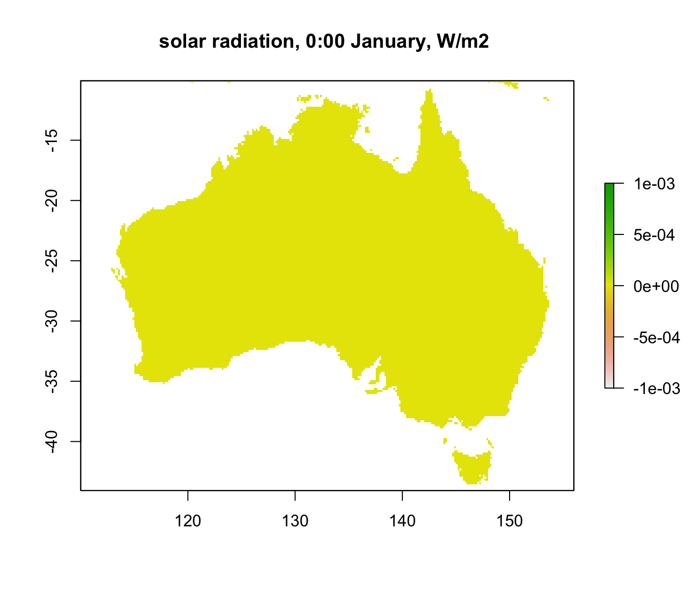
Well, that’s not very interesting is it? This is because we plotted layer 1 which is midnight. Let’s plot layer 13, which is 12 noon, instead.

Now we can see a wide range of values, from near 1000 \(W\:m^{-2}\) in central Australia down to just over 700 in the far north and south of the country. You can clearly see the effect of cloud cover during the wet season in the ‘Top End’ of Australia.
You may have also noticed the somewhat blocky appearance of the layer. This is because the aerosol and cloud cover layers are a coarser resolution than the rest of the input grids. In fact, there is a big increase in the aerosol grid (and hence decrease in the solar radiation) over central Australia which has been manually reduced in this data set from the original microclim data set.
Now let’s extract and plot 24 hours of data from a particular location. We’ll use the same location we used in Prac 1, i.e. a place in the Flinders Ranges of South Australia. First we’ll plot the chosen location on the map. Then, we once again use the ‘raster’ package function extract, which we met in Prac 1, to get the data for that point across all 24 layers.
lon.lat = cbind(138,-32) # define the longitude and latitude
points(lon.lat, cex=1.5, pch=16, col='black') # note that cex specifies the point size 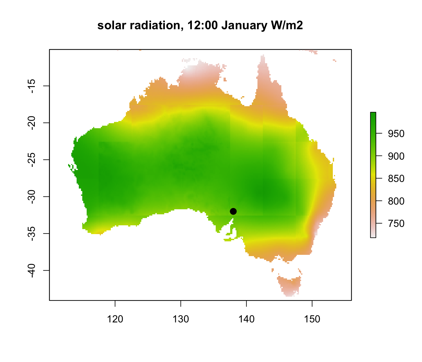
# extract data for all layers in 'solar' at location 'lon.lat'
solar.hr = extract(solar, lon.lat)
solar.hr = t(solar.hr) # transpose the values, in preparation for the plot command
hrs = seq(0,23) # create a sequence of hours
# plot solar radiation as a function of hour, as a line graph (using type = 'l')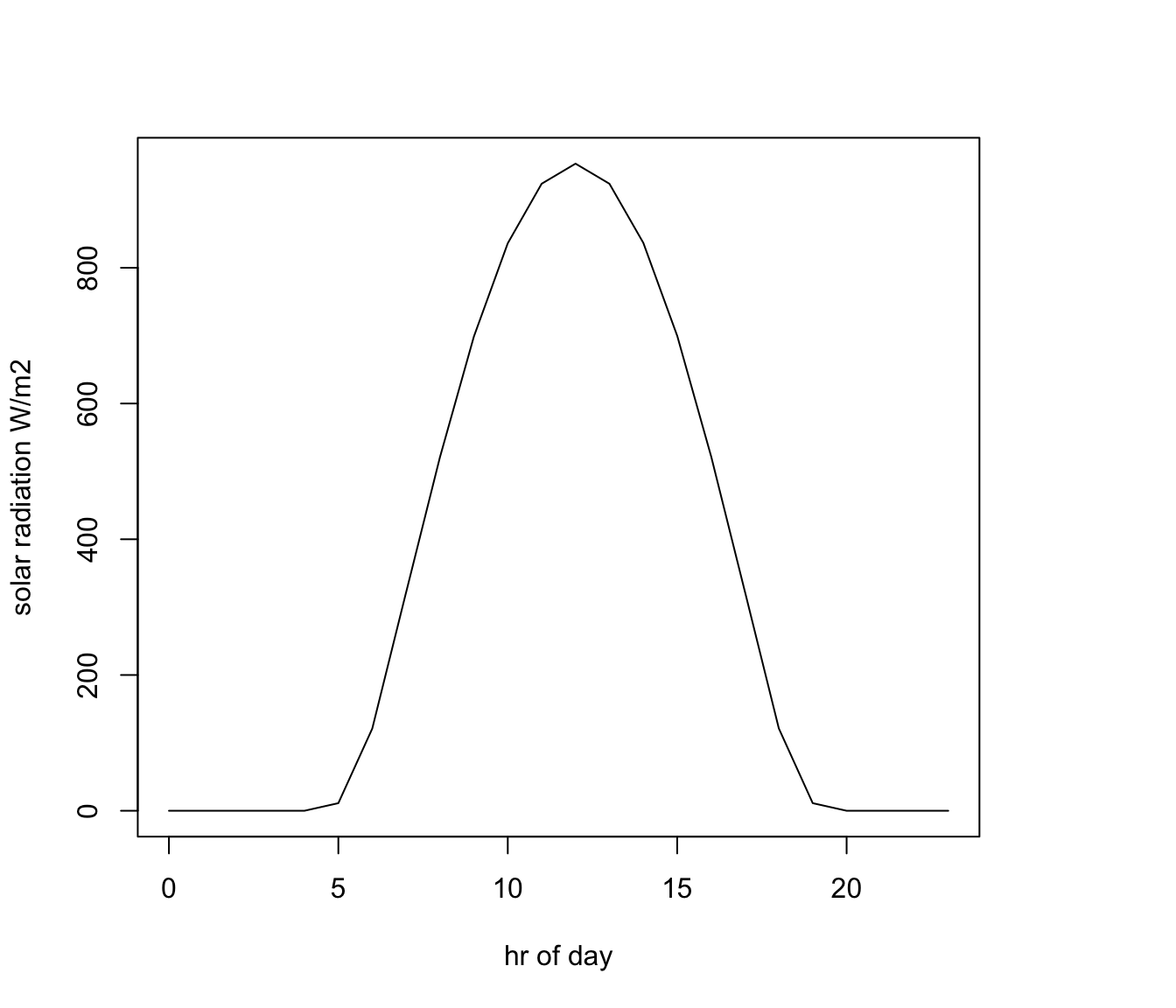
15.5 Zenith Angle
The solar radiation layers are for flat ground but often we need to compute radiation at different angles relative to the sun’s rays, for which we need to know the zenith angle. This is the angle the sun is in the sky relative to a point directly overhead (so a zenith angle of 0 degrees is when the sun is directly overhead and 90 degrees or greater is below the horizon). This can also tell us about twilight hours, which is when there is still some solar radiation present but the zenith angle is greater than or equal to 90 (the sun has just disappeared).
The code chunk below reads in and plots the zenith angles for midday for summer and winter in Australia.
month<-1 # choose which month you want, 1 or 7 (i.e. Jan or Jun)
# read the file into memory
ZEN_jan<-brick(paste0(path,"zenith_angle/ZEN_",month,".nc"))
month<-7 # choose which month you want, 1 or 7 (i.e. Jan or Jun)
# read the file into memory
ZEN_jul<-brick(paste0(path,"zenith_angle/ZEN_",month,".nc"))
par(mfrow = c(1,2)) # set to plot 1 row of 2 panels
plot(ZEN_jan[[13]],main = "zenith angle, deg, 12:00 January", zlim = c(0,70))
plot(ZEN_jul[[13]],main = "zenith angle, deg, 12:00 July", zlim = c(0,70))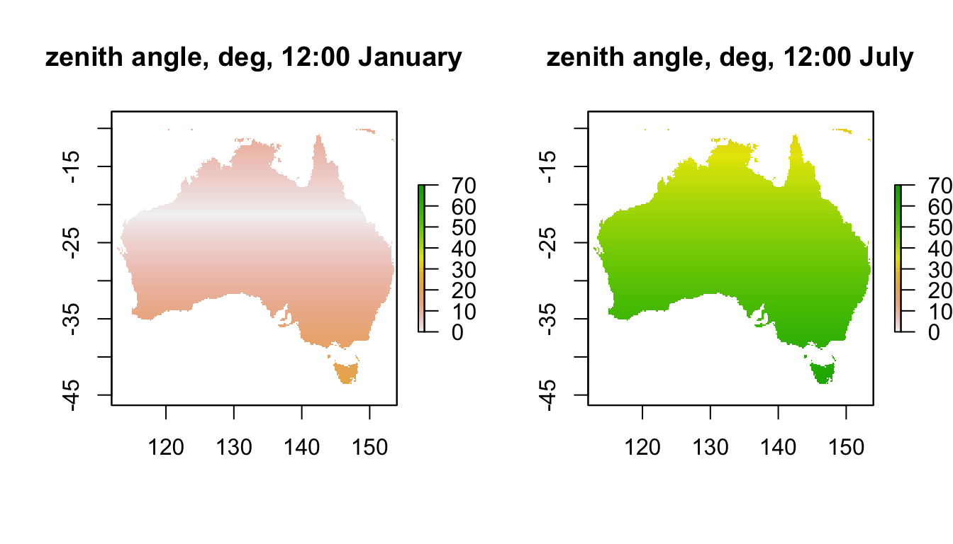
Note how the sun is almost directly overhead at a band at a latitude 23.5 degrees south in January. What is this important latitude called? Note how low the sun is in July, especially in Tasmania where it can be as low as 65 degrees at midday.
If we look at the zenith angles through the day at our Flinders Ranges site in the two months, we get the following:
# extract data for all layers in 'ZEN_jan' at location 'lon.lat'
ZEN_jan.hr = t(extract(ZEN_jan, lon.lat))
# extract data for all layers in 'ZEN_jul' at location 'lon.lat'
ZEN_jul.hr = t(extract(ZEN_jul, lon.lat))

par(mfrow = c(1,1)) # revert to 1 panel
# plot zenith angle in January as a function of hour, as a line graph (using type = 'l'),
# in red
plot(ZEN_jan.hr ~ hrs, type = 'l', ylim=c(0,90), ylab = "solar zenith angle, degrees",
     xlab = "hr of day", col = 'red')
# plot zenith angle in July as a function of hour, as a line graph (using type = 'l'),
# with January in red and June in blue.
points(ZEN_jul.hr ~ hrs, type = 'l', col = 'blue')
legend(0, 60, c("January", "July"), col = c("red", "blue"), lty=c(1), bty = "n")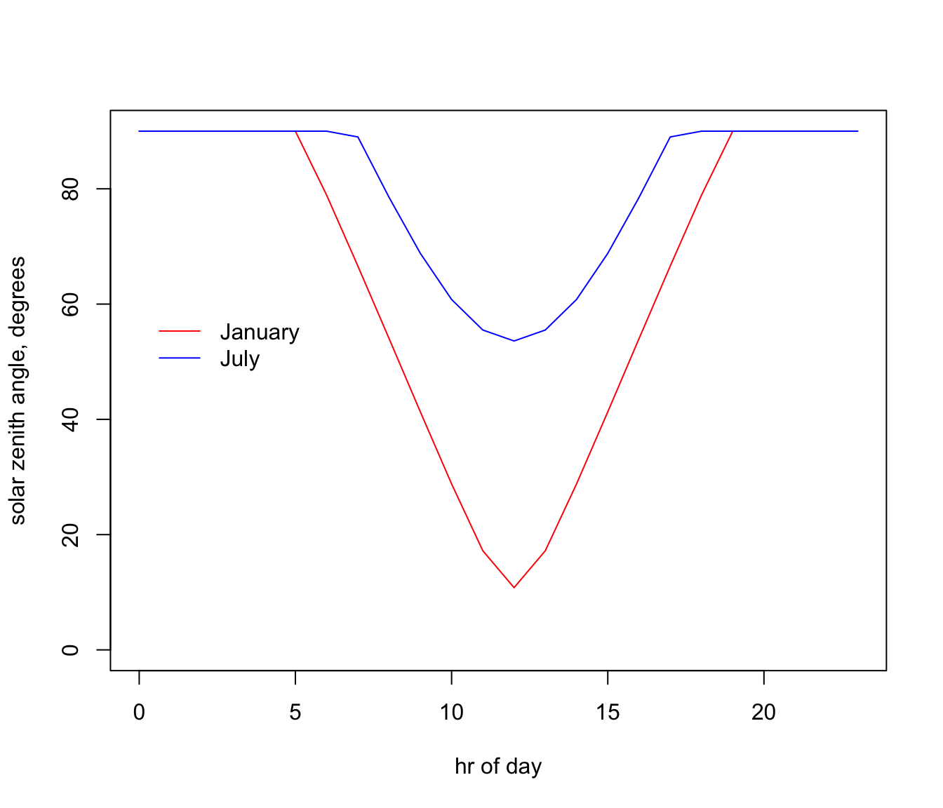
15.6 Wind Speed
For wind speed, notice how there are values for two heights, 1cm and 10m. The 10m value is what comes from the New et al. (2002) data set and is the height of the weather station wind speed measurements used by New et al. (2002) to interpolate the wind speed grids. But 10m isn’t a particularly useful height for calculating organismal heat and water budgets (well, except for trees and dinosaurs). The 1cm height was arbitrarily chosen as a useful general height at which to have microclimatic data, but this can be adjusted to different heights as discussed in Kearney et al. (2014).
The code chunk below reads in and plots the wind speed in January and July at midday at the two different heights.
month<-1 # choose which month you want, 1 or 7 (i.e. Jan or Jun)
# read the files into memory
V10m_jan<-brick(paste0(path,"wind_speed_ms_10m/V10m_",month,".nc"))
V1cm_jan<-brick(paste0(path,"wind_speed_ms_1cm/V1cm_",month,".nc"))
month<-7 # choose which month you want, 1 or 7 (i.e. Jan or Jun)
V10m_jul<-brick(paste0(path,"wind_speed_ms_10m/V10m_",month,".nc"))
V1cm_jul<-brick(paste0(path,"wind_speed_ms_1cm/V1cm_",month,".nc"))

par(mfrow = c(2,2)) # set to plot 2 rows of 2 panels
plot(V10m_jan[[13]],main = "wind speed 10m, 12:00 January, m/s", zlim = c(0,8))
plot(V1cm_jan[[13]],main = "wind speed 1cm, 12:00 January, m/s", zlim = c(0,2))
plot(V10m_jul[[13]],main = "wind speed 10m, 12:00 July, m/s", zlim = c(0,8))
plot(V1cm_jul[[13]],main = "wind speed 1cm, 12:00 July, m/s", zlim = c(0,2))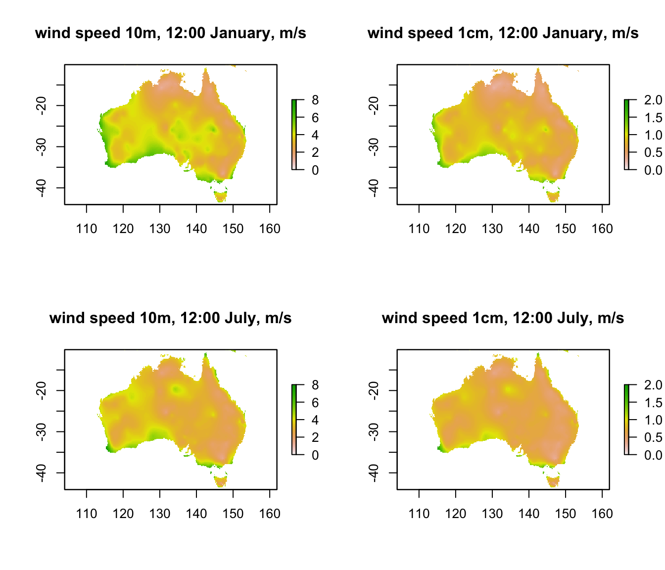
You can see that the coastal areas often have higher wind speeds, especially on the west coast in January. Note also the very big drop in wind speed as you go from 10m to 1cm (check the scale bars). The next code chunk plots the hourly wind speed at the Flinders Ranges site at each height in each month. Here, the magnitude of the difference between the heights is even clearer. Note also that there is no diurnal variation in wind speed in this data set because the New et al. (2002) data set does not have min/max wind speed but rather just the average daily wind speed.
# extract data for all layers in 'V10m_jan' at location 'lon.lat'
V10m_jan.hr = t(extract(V10m_jan, lon.lat))
# extract data for all layers in 'V10m_jan' at location 'lon.lat'
V1cm_jan.hr = t(extract(V1cm_jan, lon.lat))
# extract data for all layers in 'V1cm_jan' at location 'lon.lat'
V10m_jul.hr = t(extract(V10m_jul, lon.lat))
# extract data for all layers in 'V1cm_jan' at location 'lon.lat'
V1cm_jul.hr = t(extract(V1cm_jul, lon.lat))

# plot wind speed at 10m in January as a function of hour, as a line graph (using type = 'l'), in red
par(mfrow = c(1,2)) # set to plot 1 row of 2 panels
plot(V10m_jan.hr ~ hrs, type = 'l', main = "January", ylab = "wind speed, m/s", xlab = "hr of day", col = 'red', ylim = c(0,5))
# plot wind speed at 1cm in January as a function of hour, as a line graph (using type = 'l'),
# with 10m in red and 1cm in blue.
points(V1cm_jan.hr ~ hrs, type = 'l', col = 'blue')

# plot wind speed at 10m in January as a function of hour, as a line graph (using type = 'l'), in red
plot(V10m_jul.hr ~ hrs, type = 'l', main = "July", ylab = "wind speed, m/s", xlab = "hr of day", col = 'red', ylim = c(0,5))
# plot wind speed at 1cm in July as a function of hour, as a line graph (using type = 'l'),
# with 10m in red and 1cm in blue.
points(V1cm_jul.hr ~ hrs, type = 'l', col = 'blue')

legend(0, 5, c("10m", "1cm"), col = c("red", "blue"), lty=c(1), bty = "n")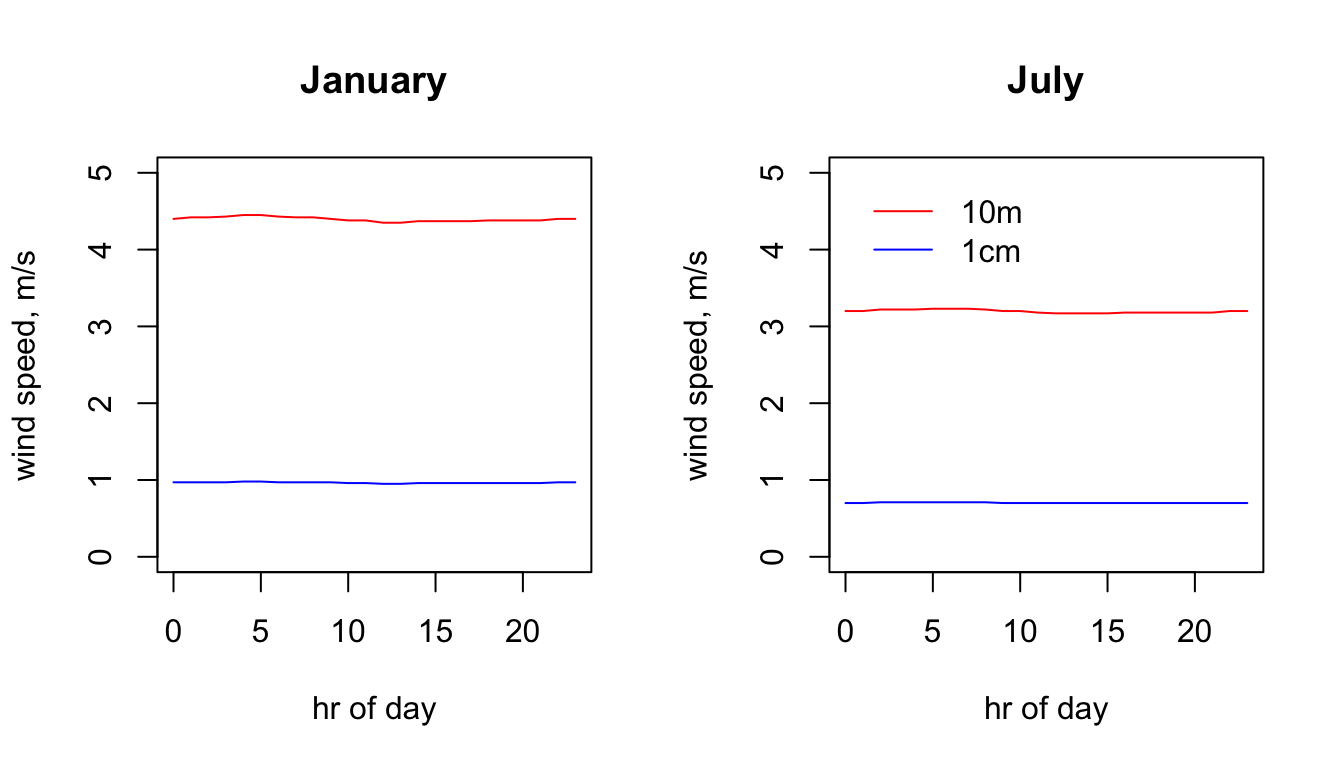
15.7 Air Temperature
As with wind speed, there are two folders for air temperature, at different heights above the ground. In the case of air temperature, the height of the measurements in the weather station data used by New et al. (2002) was 120cm. And, as for wind speed, the microclimate model has been used to estimate values for 1cm above the ground.
Note also that, for the 1cm air temperatures, there are sub-folders specifying the substrate type and the shade level. This is because the estimated value of air temperature at this height is dependent on what shade and substrate type were used in the simulation. You have only been provided with two shade levels, 0 and 100%.
The next code chunk plots the air temperature at 120 cm for the two months at midday.
month<-1 # choose which month you want, 1 or 7 (i.e. Jan or Jun)
# read the file into memory
Tair120cm_jan<-brick(paste0(path,"air_temperature_degC_120cm/TA120cm_",month,".nc"))

month<-7 # choose which month you want, 1 or 7 (i.e. Jan or Jun)
# read the file into memory
Tair120cm_jul<-brick(paste0(path,"air_temperature_degC_120cm/TA120cm_",month,".nc"))

par(mfrow = c(1,2)) # set to plot 1 row of 2 panels
plot(Tair120cm_jan[[13]],main = "Tair 120cm, 12:00 January, deg C", zlim = c(0,40))
plot(Tair120cm_jul[[13]],main = "Tair 120cm, 12:00 July, deg C", zlim = c(0,40))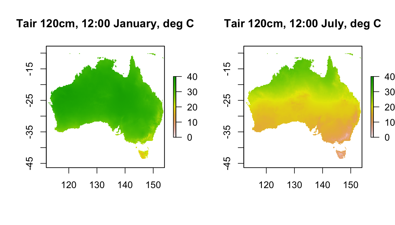
These weather station-height layers are what is typically used in correlative species distribution models.
Now we will plot the values at a 1cm height in 0% shade and in 100% shade.
month<-1 # choose which month you want, 1 or 7 (i.e. Jan or Jun)
shade <- 0 # choose which shade level you want, 0 or 100%
# read the file into memory
Tair1cm_0shade_jan<-brick(paste0(path,"air_temperature_degC_1cm/soil/",
                                 shade,"_shade/TA1cm_soil_",shade,"_",month,".nc"))

shade <- 100 # choose which shade level you want, 0 or 100%
# read the file into memory
Tair1cm_100shade_jan<-brick(paste0(path,"air_temperature_degC_1cm/soil/",
                                   shade,"_shade/TA1cm_soil_",shade,"_",month,".nc"))

month<-7 # choose which month you want, 1 or 7 (i.e. Jan or Jun)
shade <- 0 # choose which shade level you want, 0 or 100%
# read the file into memory
Tair1cm_0shade_jul<-brick(paste0(path,"air_temperature_degC_1cm/soil/",
                                 shade,"_shade/TA1cm_soil_",shade,"_",month,".nc"))

shade <- 100 # choose which month you want, 0 or 100%
# read the file into memory
Tair1cm_100shade_jul<-brick(paste0(path,"air_temperature_degC_1cm/soil/",
                                   shade,"_shade/TA1cm_soil_",shade,"_",month,".nc"))

par(mfrow = c(2,2)) # set to plot 2 rows of 2 panels
plot(Tair1cm_100shade_jan[[13]], main = "Tair 1cm 100% shade, 12:00 January, deg C", zlim = c(0,60))
plot(Tair1cm_100shade_jul[[13]], main = "Tair 1cm 100% shade, 12:00 July, deg C", zlim = c(0,60))
plot(Tair1cm_0shade_jan[[13]], main = "Tair 1cm 0% shade, 12:00 January, deg C", zlim = c(0,60))
plot(Tair1cm_0shade_jul[[13]], main = "Tair 1cm 0% shade, 12:00 July, deg C", zlim = c(0,60))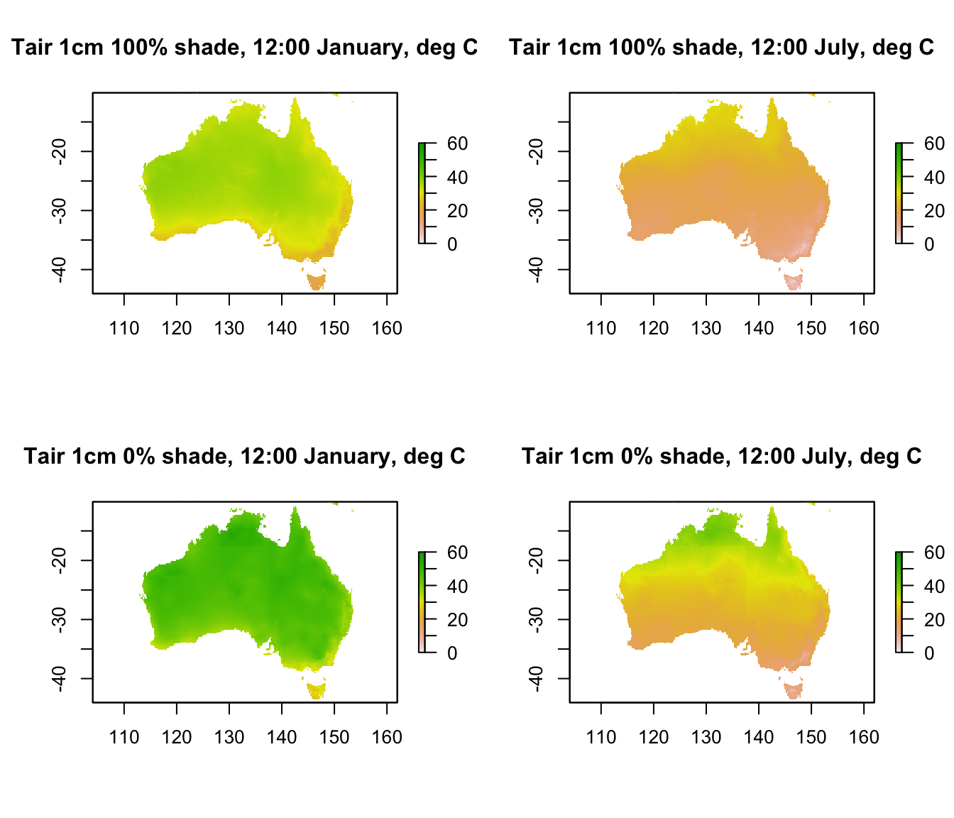
The values in 100% shade are almost identical to the 120cm values we plotted in the previous graph, and in this plot you can see that the values in 0% shade are much hotter than both the 100% shade 1cm and the 120cm air temperatures. Would this be the case at night? (take a look yourself to see the answer)
Next is some code to extract and plot the hourly values at the Flinders Ranges site for each month and height/shade level.
# extract data for all layers in 'Tair120cm_jan' at location 'lon.lat'
Tair120cm_jan.hr = t(extract(Tair120cm_jan, lon.lat))
# extract data for all layers in 'Tair120cm_jul' at location 'lon.lat'
Tair120cm_jul.hr = t(extract(Tair120cm_jul, lon.lat))
# extract data for all layers in 'Tair1cm_0shade_jan' at location 'lon.lat'
Tair1cm_0shade_jan.hr = t(extract(Tair1cm_0shade_jan, lon.lat))
# extract data for all layers in 'Tair1cm_0shade_jul' at location 'lon.lat'
Tair1cm_0shade_jul.hr = t(extract(Tair1cm_0shade_jul, lon.lat))
# extract data for all layers in 'Tair1cm_100shade_jan' at location 'lon.lat'
Tair1cm_100shade_jan.hr = t(extract(Tair1cm_100shade_jan, lon.lat))
# extract data for all layers in 'Tair1cm_100shade_jul' at location 'lon.lat'
Tair1cm_100shade_jul.hr = t(extract(Tair1cm_100shade_jul, lon.lat))

# plot air temperature at 120cm in January as a function of hour,
# as a line graph (using type = 'l'), in black
par(mfrow = c(1,2)) # set to plot 1 row of 2 panels
plot(Tair120cm_jan.hr ~ hrs, type = 'l', main = "January",
     ylab = "air temperature, deg C", xlab = "hr of day", col = 'black', ylim = c(0,45))
# plot air temperature at 1cm in 0% shade in January as a function of hour,
# as a line graph (using type = 'l'), in red.
points(Tair1cm_0shade_jan.hr ~ hrs, type = 'l', col = 'red')
# plot air temperature at 1cm in 100% shade January as a function of hour,
# as a line graph (using type = 'l'), in blue.
points(Tair1cm_100shade_jan.hr ~ hrs, type = 'l', col = 'blue')

# plot air temperature at 120cm in July as a function of hour,
# as a line graph (using type = 'l'), in black
plot(Tair120cm_jul.hr ~ hrs, type = 'l', main = "July",
     ylab = "air temperature, deg C", xlab = "hr of day", col = 'black', ylim = c(0,45))
# plot air temperature at 1cm in 0% shade in July as a function of hour,
# as a line graph (using type = 'l'), in red.
points(Tair1cm_0shade_jul.hr ~ hrs, type = 'l', col = 'red')
# plot air temperature at 1cm in 100% shade July as a function of hour,
# as a line graph (using type = 'l'), in blue.
points(Tair1cm_100shade_jul.hr ~ hrs, type = 'l', col = 'blue')

legend(0, 45, c("120cm", "1cm, 100% shade", "1cm, 0% shade"),
       col = c("black", "blue", "red"), lty=c(1, 1, 1), bty = "n")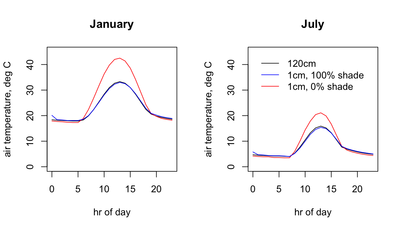
15.8 Sky Temperature
The sky temperature is the temperature you would measure if you pointed an infra-red thermometer at the sky. It is used to compute the downward flux of infra-red radiation and is estimated by the microclimate model as function of air temperature, cloud cover, relative humidity and shade.
The code below shows the values for each month and shade level at midnight. Note the extremely cold skies in central Australia in July in 0% shade, where the cloud cover and relative humidity are very low.
month<-1 # choose which month you want, 1 or 7 (i.e. Jan or Jun)
shade <- 0 # choose which month you want, 0 or 100%
Tsky_0shade_jan<-brick(paste0(path,"sky_temperature_degC/",shade,"_shade/TSKY_",
                              shade,"_",month,".nc")) # read the file into memory
shade <- 100 # choose which month you want, 0 or 100%
Tsky_100shade_jan<-brick(paste0(path,"sky_temperature_degC/",shade,"_shade/TSKY_",
                                shade,"_",month,".nc")) # read the file into memory
month<-7 # choose which month you want, 1 or 7 (i.e. Jan or Jun)
shade <- 0 # choose which month you want, 0 or 100%
Tsky_0shade_jul<-brick(paste0(path,"sky_temperature_degC/",shade,"_shade/TSKY_",
                              shade,"_",month,".nc")) # read the file into memory
shade <- 100 # choose which month you want, 0 or 100%
Tsky_100shade_jul<-brick(paste0(path,"sky_temperature_degC/",shade,"_shade/TSKY_",
                                shade,"_",month,".nc")) # read the file into memory

par(mfrow = c(2,2)) # set to plot 2 rows of 2 panels
plot(Tsky_0shade_jan[[1]],main = "Tsky 0% shade, 0:00 January, deg C", zlim = c(-20,20))
plot(Tsky_100shade_jan[[1]],main = "Tsky 100% shade, 0:00 January, deg C", zlim = c(-20,20))
plot(Tsky_0shade_jul[[1]],main = "Tsky 0% shade, 0:00 July, deg C", zlim = c(-20,20))
plot(Tsky_100shade_jul[[1]],main = "Tsky 100% shade, 0:00 July, deg C", zlim = c(-20,20))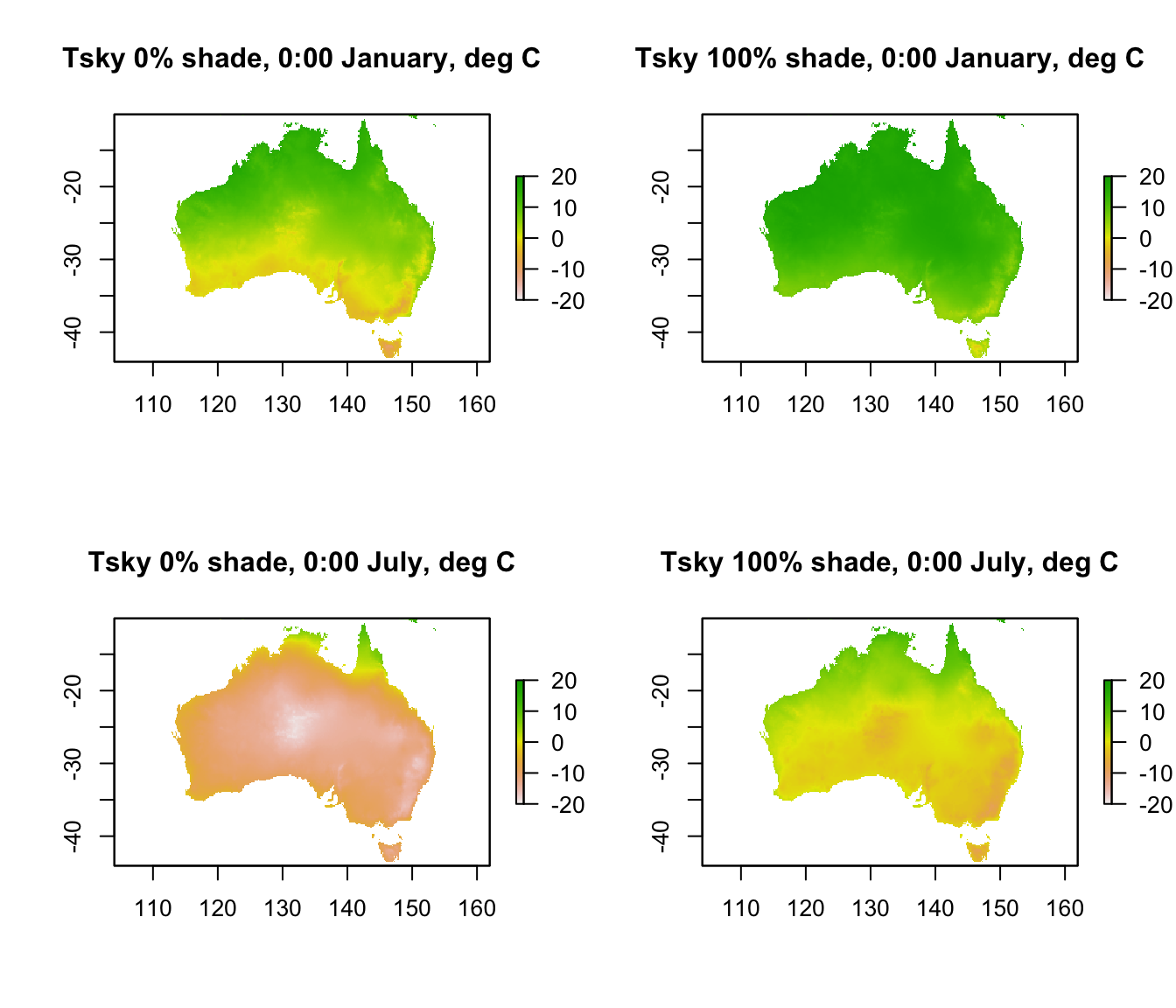
Here is the 24 hr pattern of sky temperature for the Flinders Ranges site each season for each shade level.
# extract data for all layers in 'Tsky_0shade_jan' at location 'lon.lat'
Tsky_0shade_jan.hr = t(extract(Tsky_0shade_jan, lon.lat))
# extract data for all layers in 'Tsky_0shade_jul' at location 'lon.lat'
Tsky_0shade_jul.hr = t(extract(Tsky_0shade_jul, lon.lat))
# extract data for all layers in 'Tsky_100shade_jan' at location 'lon.lat'
Tsky_100shade_jan.hr = t(extract(Tsky_100shade_jan, lon.lat))
# extract data for all layers in 'Tsky_100shade_jul' at location 'lon.lat'
Tsky_100shade_jul.hr = t(extract(Tsky_100shade_jul, lon.lat))

par(mfrow = c(1,2)) # set to plot 1 row of 2 panels
# plot sky temperature in 0% shade in January as a function of hour,
# as a line graph (using type = 'l'), in blue.
plot(Tsky_0shade_jan.hr ~ hrs, type = 'l', main = "Sky Temperature, January",
     ylab = "air temperature, deg C", xlab = "hr of day", col = 'blue', ylim = c(-20,30))
# plot sky temperature in 100% shade January as a function of hour,
# as a line graph (using type = 'l'), in red.
points(Tsky_100shade_jan.hr ~ hrs, type = 'l', col = 'red')

# plot sky temperature in 0% shade in July as a function of hour,
# as a line graph (using type = 'l'), in blue.
plot(Tsky_0shade_jul.hr ~ hrs, type = 'l', main = "Sky Temperature, July",
     ylab = "air temperature, deg C", xlab = "hr of day", col = 'blue', ylim = c(-20,30))
# plot sky temperature in 100% shade July as a function of hour, as a line graph (using type = 'l'),
# in red.
points(Tsky_100shade_jul.hr ~ hrs, type = 'l', col = 'red')

legend(0, 30, c("0% shade","100% shade"), col = c("red", "blue"), lty=c(1), bty = "n")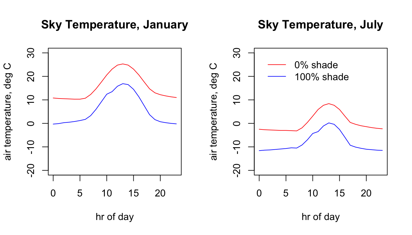
15.9 Relative Humidity
Relative humidity, similar to air temperature, is measured at 120cm and has been estimated by the microclimate model at 1cm. In the estimation, the absolute amount of water in the air has been assumed constant, and the relative humidity has been adjusted for the 1cm air temperature (remember, relative humidity is the amount of water the air is holding relative to what it could if it were saturated at that temperature, and as temperature goes up it can hold more water at saturation). Thus, we have estimates specific to soil type and shade level, as for air temperature.
Here is what the data look like at midday for each month at 120cm. You can see the strong seasonal effect in northern and southern Australia, with the humid/wet season occurring at different times of year.
month<-1 # choose which month you want, 1 or 7 (i.e. Jan or Jun)
# read the file into memory
RH120cm_jan<-brick(paste0(path,"relative_humidity_pct_120cm/RH120cm_",month,".nc"))

month<-7 # choose which month you want, 1 or 7 (i.e. Jan or Jun)
# read the file into memory
RH120cm_jul<-brick(paste0(path,"relative_humidity_pct_120cm/RH120cm_",month,".nc"))

par(mfrow = c(1,2)) # set to plot 1 row of 2 panels
plot(RH120cm_jan[[13]],main = "RH 120cm, 12:00 January, %", zlim = c(0,70))
plot(RH120cm_jul[[13]],main = "RH 120cm, 12:00 July, %", zlim = c(0,70))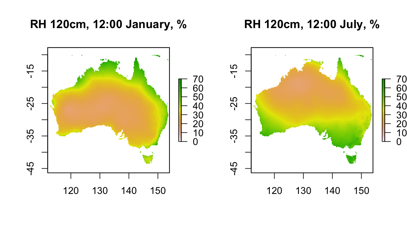
In comparison, here is the data for 1cm in 0% shade (100% shade at 1cm will be similar to 120cm, as we saw above for air temperature). Note how much lower the relative humidity is near the ground at this time of day.
month<-1 # choose which month you want, 1 or 7 (i.e. Jan or Jun)
shade <- 0 # choose which month you want, 0 or 100%
# read the file into memory
RH1cm_0shade_jan<-brick(paste0(path,"relative_humidity_pct_1cm/soil/",
                               shade,"_shade/RH1cm_soil_",shade,"_",month,".nc"))

month<-7 # choose which month you want, 1 or 7 (i.e. Jan or Jun)
# read the file into memory
RH1cm_0shade_jul<-brick(paste0(path,"relative_humidity_pct_1cm/soil/",
                               shade,"_shade/RH1cm_soil_",shade,"_",month,".nc"))

shade <- 100 # choose which month you want, 0 or 100%
# read the file into memory
RH1cm_100shade_jan<-brick(paste0(path,"relative_humidity_pct_1cm/soil/",
                                 shade,"_shade/RH1cm_soil_",shade,"_",month,".nc"))

month<-7 # choose which month you want, 1 or 7 (i.e. Jan or Jun)
# read the file into memory
RH1cm_100shade_jul<-brick(paste0(path,"relative_humidity_pct_1cm/soil/",
                                 shade,"_shade/RH1cm_soil_",shade,"_",month,".nc"))

par(mfrow = c(1,2)) # set to plot 2 rows of 2 panels
plot(RH1cm_0shade_jan[[13]],main = "RH 1cm 0% shade, 12:00 Jan, %", zlim = c(0,70))
plot(RH1cm_0shade_jul[[13]],main = "RH 1cm 0% shade, 12:00 Jul, %", zlim = c(0,70))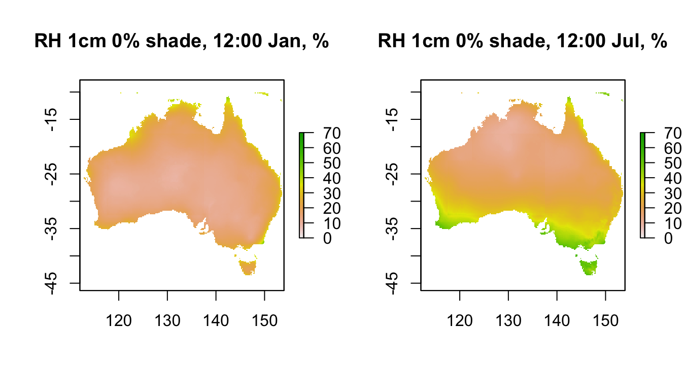
Here is the 24hr profile for relative humidity at the Flinders Ranges site.
# extract data for all layers in 'RH120cm_jan' at location 'lon.lat'
RH120cm_jan.hr = t(extract(RH120cm_jan, lon.lat))

# extract data for all layers in 'RH120cm_jul' at location 'lon.lat'
RH120cm_jul.hr = t(extract(RH120cm_jul, lon.lat))

# extract data for all layers in 'RH1cm_0shade_jan' at location 'lon.lat'
RH1cm_0shade_jan.hr = t(extract(RH1cm_0shade_jan, lon.lat))

# extract data for all layers in 'RH1cm_0shade_jul' at location 'lon.lat'
RH1cm_0shade_jul.hr = t(extract(RH1cm_0shade_jul, lon.lat))

# extract data for all layers in 'RH1cm_100shade_jan' at location 'lon.lat'
RH1cm_100shade_jan.hr = t(extract(RH1cm_100shade_jan, lon.lat))

# extract data for all layers in 'RH1cm_100shade_jul' at location 'lon.lat'
RH1cm_100shade_jul.hr = t(extract(RH1cm_100shade_jul, lon.lat))

par(mfrow = c(1,2)) # set to plot 1 row of 2 panels
# plot relative humidity at 120cm in January as a function of hour,
# as a line graph (using type = 'l'), in black
plot(RH120cm_jan.hr ~ hrs, type = 'l', main = "January", ylab = "relative humidity, %",
     xlab = "hr of day", col = 'black', ylim = c(0,100))
# plot relative humidity at 1cm in 0% shade in January as a function of hour,
# as a line graph (using type = 'l'), in red.
points(RH1cm_0shade_jan.hr ~ hrs, type = 'l', col = 'red')
# plot relative humidity at 1cm in 100% shade January as a function of hour,
# as a line graph (using type = 'l'), in blue.
points(RH1cm_100shade_jan.hr ~ hrs, type = 'l', col = 'blue')

# plot relative humidity at 120cm in July as a function of hour,
# as a line graph (using type = 'l'), in black
plot(RH120cm_jul.hr ~ hrs, type = 'l', main = "July", ylab = "relative humidity, %",
     xlab = "hr of day", col = 'black', ylim = c(0,100))
# plot relative humidity at 1cm in 0% shade in July as a function of hour,
# as a line graph (using type = 'l'), in red.
points(RH1cm_0shade_jul.hr ~ hrs, type = 'l', col = 'red')
# plot relative humidity at 1cm in 100% shade July as a function of hour,
# as a line graph (using type = 'l'), in blue.
points(RH1cm_100shade_jul.hr ~ hrs, type = 'l', col = 'blue')

legend(-2, 40, c("120cm", "1cm, 100% shade", "1cm, 0% shade"), col = c("black", "blue", "red"),
       lty=c(1, 1, 1), bty = "n")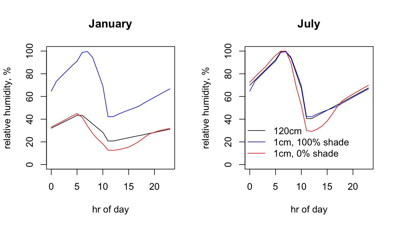
15.10 Soil Temperature
The final environmental data set in microclim is for substrate temperature. As with air temperature and relative humidity at 1cm, there are separate sets for each substrate type and shade level. Indeed, it is the thermal properties specified for each substrate type (thermal conductivity, specific heat capacity and density) that drive the substrate-specific differences in air temperature and relative humidity at 1cm. In this case we only have access to the soil substrate type.
There are 9 different depths at which soil temperature has been predicted by the microclimate model - 0, 2.5, 5, 10, 15, 20, 30, 50 and 100 cm (note the 2.5 cm layer is named 3cm, but it is for 2.5!). Let’s take a look at the 0cm depth layers in each month at midday across Australia.
month<-1 # choose which month you want, 1 or 7 (i.e. Jan or Jun)
shade <- 0 # choose which month you want, 0 or 100%
# read the file into memory
D0cm_0shade_jan<-brick(paste0(path,"substrate_temperature_degC/soil/",
                              shade,"_shade/D0cm_soil_",shade,"_",month,".nc"))

shade <- 100 # choose which month you want, 0 or 100%
# read the file into memory
D0cm_100shade_jan<-brick(paste0(path,"substrate_temperature_degC/soil/",
                                shade,"_shade/D0cm_soil_",shade,"_",month,".nc"))

month<-7 # choose which month you want, 1 or 7 (i.e. Jan or Jun)
shade <- 0 # choose which month you want, 0 or 100%
# read the file into memory
D0cm_0shade_jul<-brick(paste0(path,"substrate_temperature_degC/soil/",
                              shade,"_shade/D0cm_soil_",shade,"_",month,".nc"))

shade <- 100 # choose which month you want, 0 or 100%
# read the file into memory
D0cm_100shade_jul<-brick(paste0(path,"substrate_temperature_degC/soil/",
                                shade,"_shade/D0cm_soil_",shade,"_",month,".nc"))

par(mfrow = c(2,2)) # set to plot 2 rows of 2 panels
plot(D0cm_100shade_jan[[13]],main = "Tsoil 0cm 100% shade, 12:00 Jan, deg C", zlim = c(0,80))
plot(D0cm_100shade_jul[[13]],main = "Tsoil 0cm 100% shade, 12:00 Jul, deg C", zlim = c(0,80))
plot(D0cm_0shade_jan[[13]],main = "Tsoil 0cm 0% shade, 12:00 Jan, deg C", zlim = c(0,80))
plot(D0cm_0shade_jul[[13]],main = "Tsoil 0cm 0% shade, 12:00 Jul, deg C", zlim = c(0,80))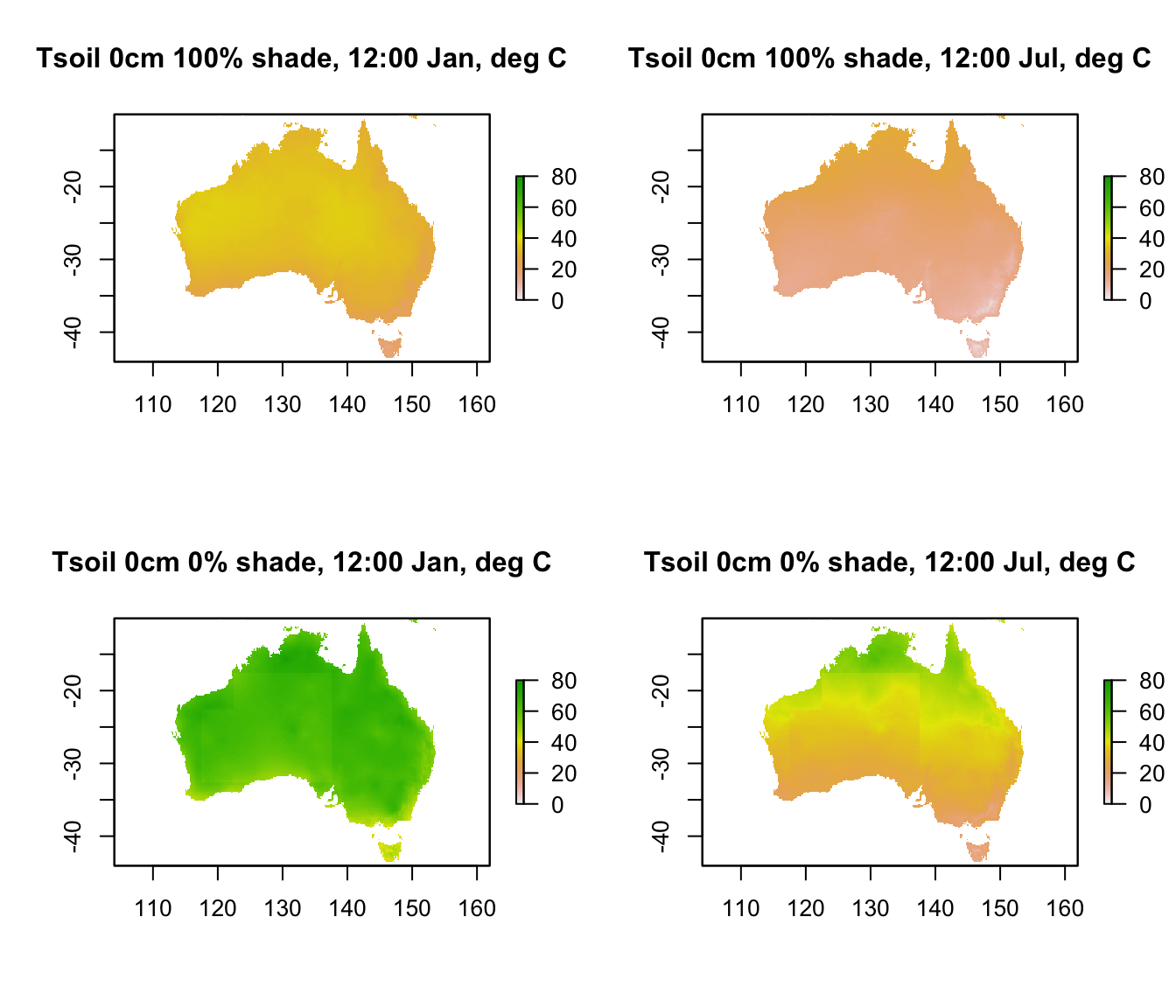
Note that there is a range of almost 80\(^\circ\)C in predicted soil surface temperature across Australia. Let’s go down 5 cm into the ground and see the difference in temperature, keeping the scale the same.
month<-1 # choose which month you want, 1 or 7 (i.e. Jan or Jun)
shade <- 0 # choose which month you want, 0 or 100%
# read the file into memory
D5cm_0shade_jan<-brick(paste0(path,"substrate_temperature_degC/soil/",
                              shade,"_shade/D5cm_soil_",shade,"_",month,".nc"))

shade <- 100 # choose which month you want, 0 or 100%
# read the file into memory
D5cm_100shade_jan<-brick(paste0(path,"substrate_temperature_degC/soil/",
                                shade,"_shade/D5cm_soil_",shade,"_",month,".nc"))

month<-7 # choose which month you want, 1 or 7 (i.e. Jan or Jun)
shade <- 0 # choose which month you want, 0 or 100%
# read the file into memory
D5cm_0shade_jul<-brick(paste0(path,"substrate_temperature_degC/soil/",
                              shade,"_shade/D5cm_soil_",shade,"_",month,".nc"))

shade <- 100 # choose which month you want, 0 or 100%
# read the file into memory
D5cm_100shade_jul<-brick(paste0(path,"substrate_temperature_degC/soil/",
                                shade,"_shade/D5cm_soil_",shade,"_",month,".nc"))

par(mfrow = c(2,2)) # set to plot 2 rows of 2 panels
plot(D5cm_100shade_jan[[13]],main = "Tsoil 5cm 100% shade, 12:00 Jan, deg C", zlim = c(0,80))
plot(D5cm_100shade_jul[[13]],main = "Tsoil 5cm 100% shade, 12:00 Jul, deg C", zlim = c(0,80))
plot(D5cm_0shade_jan[[13]],main = "Tsoil 5cm 0% shade, 12:00 Jan, deg C", zlim = c(0,80))
plot(D5cm_0shade_jul[[13]],main = "Tsoil 5cm 0% shade, 12:00 Jul, deg C", zlim = c(0,80))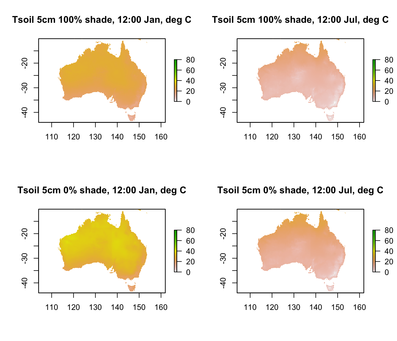
You can see that there’s a very large drop in temperature of as much as 40 degrees as you go down just 5 cm into the soil.
The next code chunk extracts the hourly temperature profile for January in 0% at the Flinders Ranges site, and then plots it
month<-1 # choose which month you want, 1 or 7 (i.e. Jan or Jun)
shade <- 0 # choose which month you want, 0 or 100%
data<-brick(paste(path,"substrate_temperature_degC/soil/",shade,
                  "_shade/D0cm_soil_",shade,"_",month,".nc",sep=""))
D0cm <- t(extract(data,lon.lat))
data<-brick(paste(path,"substrate_temperature_degC/soil/",shade,
                  "_shade/D3cm_soil_",shade,"_",month,".nc",sep=""))
D2.5cm <- t(extract(data,lon.lat))
data<-brick(paste(path,"substrate_temperature_degC/soil/",shade,
                  "_shade/D5cm_soil_",shade,"_",month,".nc",sep=""))
D5cm <- t(extract(data,lon.lat))
data<-brick(paste(path,"substrate_temperature_degC/soil/",shade,
                  "_shade/D10cm_soil_",shade,"_",month,".nc",sep=""))
D10cm <- t(extract(data,lon.lat))
data<-brick(paste(path,"substrate_temperature_degC/soil/",shade,
                  "_shade/D15cm_soil_",shade,"_",month,".nc",sep=""))
D15cm <- t(extract(data,lon.lat))
data<-brick(paste(path,"substrate_temperature_degC/soil/",shade,
                  "_shade/D20cm_soil_",shade,"_",month,".nc",sep=""))
D20cm <- t(extract(data,lon.lat))
data<-brick(paste(path,"substrate_temperature_degC/soil/",shade,
                  "_shade/D30cm_soil_",shade,"_",month,".nc",sep=""))
D30cm <- t(extract(data,lon.lat))
data<-brick(paste(path,"substrate_temperature_degC/soil/",shade,
                  "_shade/D50cm_soil_",shade,"_",month,".nc",sep=""))
D50cm <- t(extract(data,lon.lat))
data<-brick(paste(path,"substrate_temperature_degC/soil/",shade,
                  "_shade/D100cm_soil_",shade,"_",month,".nc",sep=""))
D100cm <- t(extract(data,lon.lat))

par(mfrow=c(1,1))
plot(D0cm ~ hrs,xlab = "Time of Day (hr)", ylab = "Tsoil, deg C",
     type = "l", ylim=c(0,70), main = "Soil Temperature, January")
points(D2.5cm ~ hrs,xlab = "Time of Day (hr)", col=2, type = 'l')
points(D5cm ~ hrs,xlab = "Time of Day (hr)", col=3, type = 'l')
points(D10cm ~ hrs,xlab = "Time of Day (hr)", col=4, type = 'l')
points(D15cm ~ hrs,xlab = "Time of Day (hr)", col=5, type = 'l')
points(D20cm ~ hrs,xlab = "Time of Day (hr)", col=6, type = 'l')
points(D30cm ~ hrs,xlab = "Time of Day (hr)", col=7, type = 'l')
points(D50cm ~ hrs,xlab = "Time of Day (hr)", col=8, type = 'l')
points(D100cm ~ hrs,xlab = "Time of Day (hr)",lty=2, col=9, type = 'l')

DEP <- c(0, 2.5, 5, 10, 15, 20, 30, 50, 100)
leg.txt<-paste(DEP,"cm", sep = "")
legend(1,70,lty=c(1,1,1,1,1,1,1,1,2),leg.txt,col=c(1,2,3,4,5,6,7,8,9),
       cex=1,box.lty=0)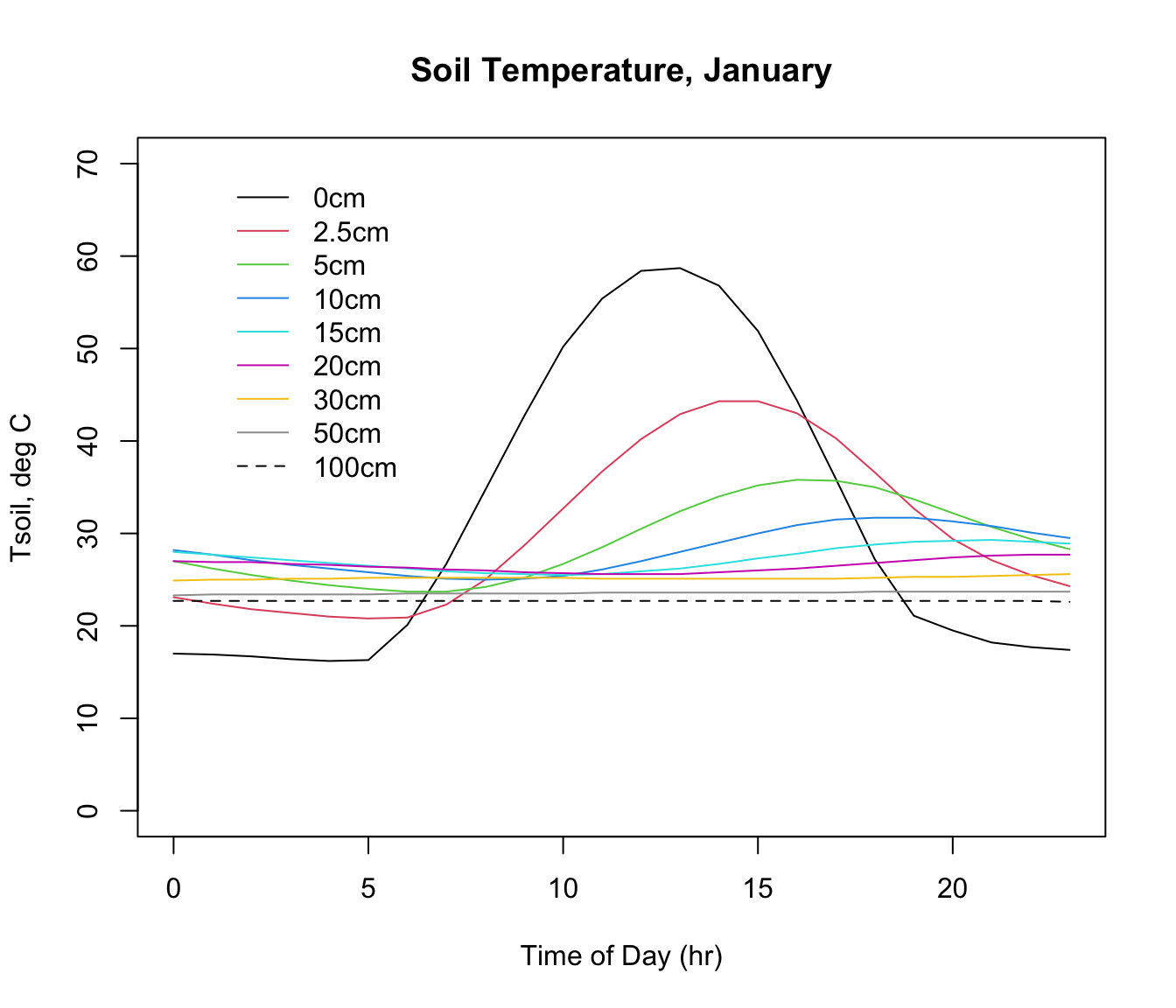
Note how the amplitude and timing of the maximum and minimum values shift with depth. The thermal profile with depth and time in the soil depends in part on the driving environmental conditions above the ground (air temperature, wind speed, radiation) but also on the thermal characteristics of the soil. This includes the moisture content, and the calculations include an estimate of soil moisture from the NOAA CPC Soil Moisture data set. The microclimate model used this soil moisture information to adjust the thermal properties of the soil at each location and month.
You can have a look at this soil temperature profile for 100% shade, or for July, by simply changing the ‘shade’ and ‘month’ values in the code chunk above. Try it, and try looking at some of these variables for other places of interest to you in Australia.
15.11 LITERATURE CITED
Kearney, M. R., A. P. Isaac, and W. P. Porter. 2014. microclim: Global estimates of hourly microclimate based on long-term monthly climate averages. Scientific Data 1:140006.
New, M., D. Lister, M. Hulme, and I. Makin. 2002. A high-resolution data set of surface climate over global land areas. Climate Research 21:1-25.
15.12 PROBLEMS
- You have also been supplied with the same set of microclimate data for North America. Take a look at it by simply altering the variable ‘path’, which we defined right at the beginning, to wherever you decompressed the North American data set archive ‘microclim_NAm.zip’. Note you’ll have to choose a new location to extract hourly data from, i.e. change the variable ‘lon.lat’.
What are some of the major differences you see between the microclimatic environments of Australia and the USA? For example, did you need to change the limits on the axes of some of the graphs?