Chapter 2 FLOOD RISK MANAGEMENT I
Integrated risk management of flood events requires complex, trans-disciplinary approaches. The module focuses on the relevant physical processes of flood risks for a comprehensive risk analysis.
2.1 Framework of Integrated Flood Risk Management
This section is based on the lecture “A Framework of Integrated Flood Risk Management”(Schanze 2016).
2.1.1 Basic terms
A flood is a temporary covering of land by water outside its normal confines.(FLOODsite-Consortium 2009)
Typology
Type of flood (site):
- Plain floods
- Flash floods
- Estuarial floods
- Coastal floods
- Pluvial floods
Cause of event:
- Cyclone rainfall floods
- Snowmelt floods
- Sea surge and tidal floods
- Urban sewer floods
- Dam break or reservoir control floods
from “Flood Protection” towards “Flood Risk Management”
Defination: The paradigm change is based on the recognition that absolute flood protection is unachievable and unsustainable, because of high costs and inherent uncertainties.
Flood risk is understood as probability of negative consequences due to floods and can only be reduced to a tolerable level.
Flood risk management considers all relevant processes of the flood hazard and the flood vulnerability to govern flood risks.
Risk = probability * (negativ) consequence [not certainly]
Flood risk = flood hazard * (exposure) * flood vulnerability
vulnerability = value/function * susceptibility * coping capacity
Risk = f(Hazard, Vulnerability)
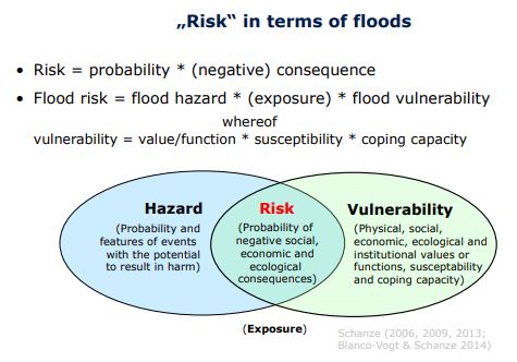
Bild aus Schatze (Schanze 2016).
Flood hazard A physical event, phenomenon or human activity with the potential to result in harm. A hazard does not necessarily lead to harm.
Hazards are normally described as the probability of flood events with a certain magnitude and other features.
Flood vulnerability Characteristic of a system that describes its potential to be harmed. It covers physical, social, economic, ecological and institutional aspects.
Areas of Vulnerability direct / indirect tangible / intangible
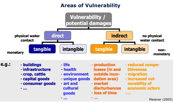
Bild aus Schatze (Schanze 2016).
2.1.2 Main causal relations within the flood risk system
Source \(\rightarrow\) pathway \(\rightarrow\) receptor \(\rightarrow\) consequence
Flood risk = f(fsource(probability, features), fpathway(inundation, attributes), freceptor(susceptibility), fconsequence(value, coping capacity))
2.1.3 Task and components of flood risk management
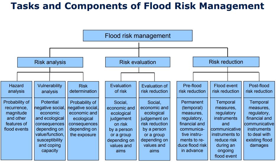
Bild aus Schatze (Schanze 2016).
Flood risk management = analysis + evaluation + reduction
Hazard analysis: Quantification of magnitude and other features.
Vulnerability analysis: Quantification and qualification of potential adverse social, economic and ecological impacts due to flooding.
Risk determination: Methofology to caculate the nature and extent of flood risk.
Evaluating risk: Methods of tolerability aversion, sustainability and so forth depending on individual or collective interest, values and aims.
Evaluating risk reduction: Individual measures and instruments in terms of their intended performance and their relation to side-effects.
Pre-flood risk reduction: Measures and instruments including their operationalisation for modeling resulting risks ex ante and the planning and implementation process.
Flood event risk reduction:
Post-flood risk reduction:
2.2 Rainfall climatology and Climate Change
Zusammenfassung aus (Bernhofer 2021).
2.2.1 Means and Extremes
variability
Spatial variability: smaller (regional and local) variability dominates; influences of orography, exposure to general circulation pattern and influence of temperature (latitude).
Time variability: Periodic cahnges (e.g. seasonal cycle); Aperiodic changes (e.g. short events \(\rightarrow\) high intensity)
Precipitation extremes: frequency and probability
2.2.1.1 Recurrence interval:
Pe: exceedence probability
Pc: cumulative probability, Pc = 1 - Pe
T: Return period, T = 1/Pe, indicates the expected number of years that need to be considered to find the value of the variable in study.
TU: The upper confidence of return periods can be found respectively as: TU = 1/(1-U)
TL: The lower confidence of return periods can be found respectively as: TL = 1/(1-L)
2.2.1.2 Rainfall Distribution in context
Stratiform Precipitation:
Low indensity, long lasting (> 6h), wide spread \(\rightarrow\) pre-event moisture
Convective Precipitation:
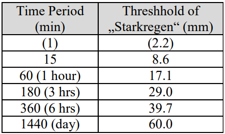
High intensity (Starkregen > 17 mm/h, Wolkenbruch > 60 mm/h), short duration (> 6 h), small scale \(\rightarrow\) flash floods
Starkniederschlag:
2.2.1.3 Statistics of precipitation extremes
Basic: long-term series of mearsured precipitation (30 a not enough, if possible 100 a or more)
Example for constructing:
- Sorting the serices (Max \(\rightarrow\) Min) per year
- Selection of the maxima of each year
- Result: a series of annual precipitation maxima
- Adaptation of theoretical distribution of extremes (Gumbel) to the measured precipitation series by regession
2.2.2 Climate Change
Background: Green House Effect
GHG(Green house gases):CO2, CH4, N2O, O3, FCCH, etc.
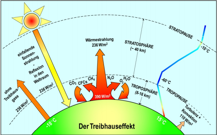
Bild aus (Bernhofer 2021).
Main excepted characterisics
Sea level rise
Higher temperatures - espesisally on land
Hydrological cycle more intense
Changes at regional level can differ (but hard to tell)
2.2.2.1 Extreme precipitation
- Statistical approach: Probability distribution fitted to the full data sample used instead
- design precipitation, SHP(D, T) = height(duration, return)
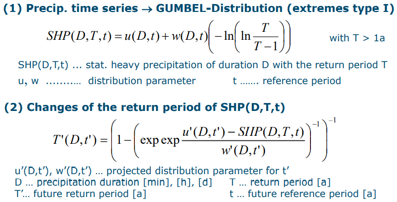
Bild aus (Bernhofer 2021).
2.3 Hydrological aspects of climate change
Zusammenfassung aus (Zimmermann 2021).
2.3.1 Snow
Snow parameters:
snow cover duration
snow cover time
continuance of the longst snow cover period (winter cover)
beginning (date) of the maximum snow vover depth
constancy of the snow cover
retention of the winter cover
maximum value of the water euivalent of the snow cover
2.3.2 Model Chain Insecurity GCM-RCM
Emissionsszenario \(\rightarrow\) Globales Klimamodell (GCM) \(\rightarrow\) Regionales Klimamodell (RCM) \(\rightarrow\) Wasserhaushaltmodell (WHM)
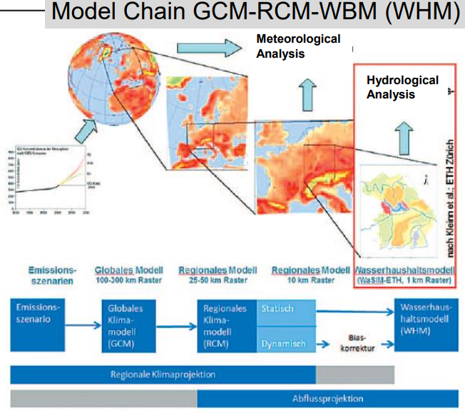
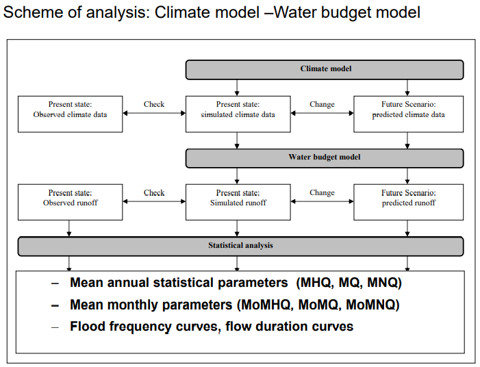
Bilder aus (Zimmermann 2021).
2.4 Physical Processes of Floods
Zusammenfassung aus (Goldberg 2021b).
2.4.1 Modern weather forecast
Computer based caculation of time-dependent change (prognosis) of all relevant atmospheric quantities (wind, temperature, humidity, density, pressure)
Solving of a system of non-linear differential equations including the above mentioned quantities
Computer simulation satrts with predescribed innitial conditions, and the caculation ends with one final solution (deterministic model)
2.4.1.1 Types and temporal ranges of weather forecast
Nowcasting: Next two hours, onlky use of observations (e.g., tracking algorithms for echoes in radar images), without representation of atmospheric physics, e.g., assumption of persistence
Short-range: 18-24 hours, daily weather
Medium-range: 3-10 days, weather for the week ahead
Long-range: > 10 days, further outlook; Comparison of cumulative precipitation forecast of one simulation for different models \(\rightarrow\) measure of uncertainty
2.4.1.2 Physical background of precipitation forecast
Cloud microphysic schemes
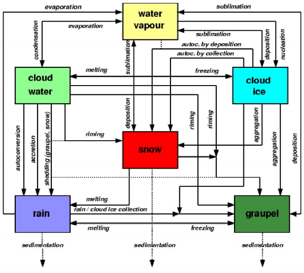
Graupel has much higher fall speeds compared to snow
Conversion processes, likesnow to graupel conversion by riming, are very difficult to parameterize but very important in convective clouds. Particle density and fall speeds are important parameters.
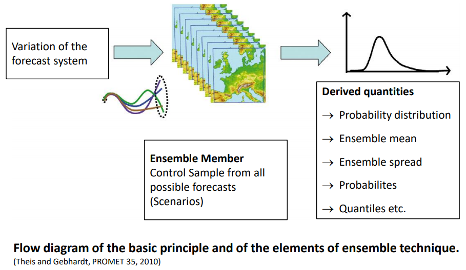
2.4.1.3 Ensemble simulation
Ensemble
estimation of the natural variance of output quantities
check of the stability of mid-range forecast
Precipitation forecast is based on ensemble siomulations and probalities
Flow diagram
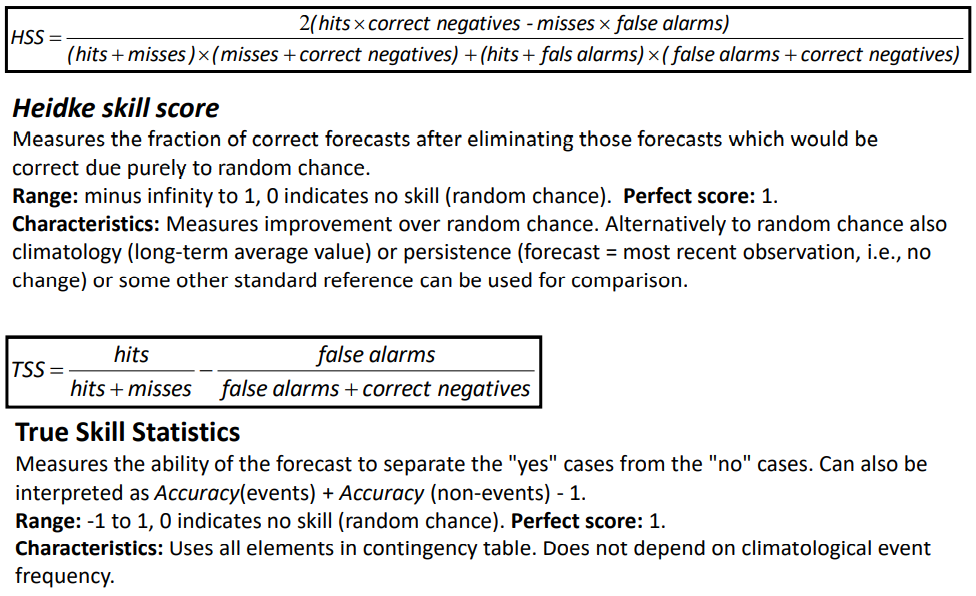
2.4.2 Evaluation of forecast quality
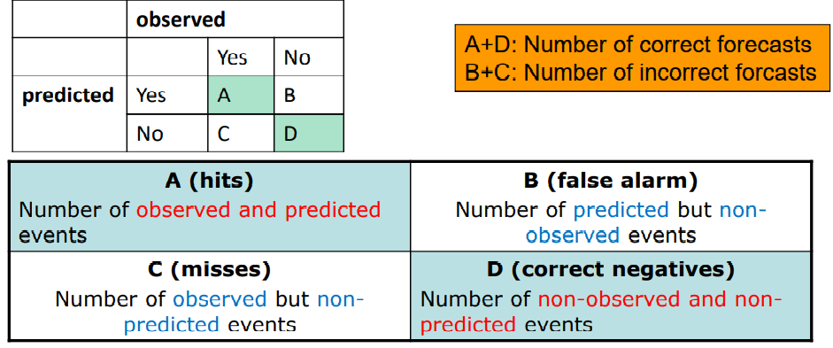
Probability of detection (Hit Rate)
Measures the fraction of observed events that were correctly predicted. Sensitive to hits, good for rare events, Ignores false alarms.
\[ POD=\frac{hits}{hits+misses} \]
Threat score (critical success index)
Measures the fraction of observed and/or forecast events that were correctly predicted. Sensitive to hits, penalizes both misses and false alarms. Does not distinguish source of forecast error. Depends on climatological frequency of events (worse scores for rarer events) since some hits can occur purely due to random chance.
\[ TS=\frac{hits}{hits+misses+false\,alarms} \]
2.4.3 Limits of weather forecast
Dependency on forecast method and forecast period
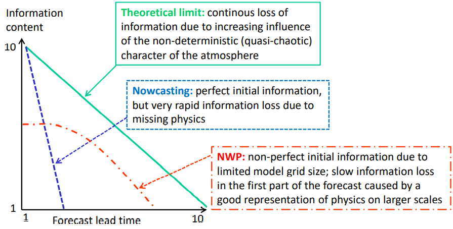
Reasons
Erroneous initial conditions for modelling (erroes in measurements and data interpolation)
Inadequate model resolution: small-scale heavy rainfall can not be simulated, orographically induced rainfall is underestimated
Inadequate model physics (convective precipitation, precipitation is only a diagnostic quantity and must be derived from other model output)
Inadequate methods of data assimilation (e.g., not all data sourecs can be considered in time)
Problems with interpretation of model results by the experts (ma made errors)
2.5 Radar
Zusammenfassung aus (Kronenberg 2021).
Radar (radio detection and ranging):
active remote sensing System
sending of micro- or radio waves (MHz- and GHz-range)
recieving of reflected radition
Radiometer (passive remote sensing system \(\rightarrow\) measurement of emitted radition)
Goals of Radar:
Distance
Speed
Form and size of obstacles
Obstacle structure/ consitency
Land surface eploration through clouds
Opareting system
Ground-based, planes
Satellite-base (orbiting satellites)
2.5.1 Radar System
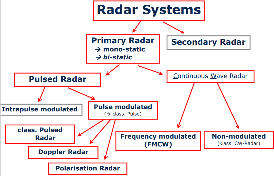
Pulsed Radar
Transmission of highly collimated EM-Waves of the antenna \(\rightarrow\) small collimated Pulses
Propagation of radation in small and long angles (Radar-Beam) with light speed \(\rightarrow\) Pulse reaches an obstacle \(\rightarrow\) Reflection (exactly Scattering)
Receiving of back scattered radition signal
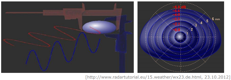
Pulse with diferent Polarisations
Quotient of horizontal to vertical reflectivity differes from the drop shape differes
large drops are flat
Doppler Radar: Measurent of radial speed
Derivation of horizontal wind speed
Wind speed is an indicator for precipitation type
Polarisation Radar: Difference of drop shape from shpere
Measure for the drop size
Derivation of precipatation \(\rightarrow\) large drops / stratiform precipitation
Estimation of radar errors:
A radar measurement is instant in time, raingauge measurement is continuous
radar detectes precipitation in a certain height above ground depending on the beam angle \(\neq\) ground precipitation
Anomalous propagation of the radar beam, due to a non standard distribution of temperature and humidity with height in the atmosphere
Pantom precipitation: multi reflection in dense clouds \(\rightarrow\) increase of signal run time \(\rightarrow\) wrong estimation of rain rates
Overestimation due to Bright-Band effect
Radar artefacts, Static and moving Clutters (Wind mills, Towers, Planes, Insects); Spokes (Completly blocked beam)
2.5.2 Radar based forecast
Nowcasting = NOW + FORECASTING
Characterisation of rainfields: size, mass, centre of gravity, aces of inertia, angle of axes, class distribution, past movment, last size difference, last mass diferencr, number of successful tracks
Extrapolation of rainfields: Linear moment, Dynamics for certainty estimate, Interpolation of image possible, Orographical effects after analysis of data
hazard, flood hazard, danger
institutional,
receptor,
impact,
collective, individual or collective
sustainability,
magnitude,
derive,
Inadequate