Week 1 Syn
| John Smith |
NA |
13 |
| Jane Doe |
12 |
5 |
| Mary Johnson |
6 |
15 |
Table 1: Typical presentation dataset.
| treatmenta |
NA |
12 |
6 |
| treatmentb |
13 |
5 |
15 |
Table 2: The same data as in Table 1 but structured differently.
| John Smith |
a |
NA |
| Jane Doe |
a |
12 |
| Mary Johnson |
a |
6 |
| John Smith |
b |
13 |
| Jane Doe |
b |
5 |
| Mary Johnson |
b |
15 |
Table 3: The same data as in Table 1 but with variables in columns and
observations in rows.
Table 5: A simple example of melting. (a) is melted with one colvar,
row, yielding the molten dataset (b). The information in each table is
exactly the same, just stored in a different way.
|
|
| A |
a |
1 |
| B |
a |
2 |
| C |
a |
3 |
| A |
b |
4 |
| B |
b |
5 |
| C |
b |
6 |
| A |
c |
7 |
| B |
c |
8 |
| C |
c |
9 |
|
| Agnostic |
27 |
34 |
60 |
81 |
76 |
137 |
| Atheist |
12 |
27 |
37 |
52 |
35 |
70 |
| Buddhist |
27 |
21 |
30 |
34 |
33 |
58 |
| Catholic |
418 |
617 |
732 |
670 |
638 |
1116 |
| Don’t know/refused |
15 |
14 |
15 |
11 |
10 |
35 |
| Evangelical Prot |
575 |
869 |
1064 |
982 |
881 |
1486 |
| Hindu |
1 |
9 |
7 |
9 |
11 |
34 |
| Historically Black Prot |
228 |
244 |
236 |
238 |
197 |
223 |
| Jehovah’s Witness |
20 |
27 |
24 |
24 |
21 |
30 |
| Jewish |
19 |
19 |
25 |
25 |
30 |
95 |
Table 4: The first ten rows of data on income and religion from the Pew
Forum. Three columns, $75{100k, $100{150k and >150k, have been
omitted.
| Agnostic |
<$10k |
27 |
| Agnostic |
$10–20k |
34 |
| Agnostic |
$20–30k |
60 |
| Agnostic |
$30–40k |
81 |
| Agnostic |
$40–50k |
76 |
| Agnostic |
$50–75k |
137 |
| Agnostic |
$75–100k |
122 |
| Agnostic |
$100–150k |
109 |
| Agnostic |
>150k |
84 |
| Agnostic |
Don’t know/refused |
96 |
Table 6: The first ten rows of the tidied Pew survey dataset on income
and religion. The column has been renamed to income, and value to freq.
| 11 |
AD |
2000 |
0 |
0 |
1 |
0 |
0 |
0 |
0 |
NA |
NA |
| 37 |
AE |
2000 |
2 |
4 |
4 |
6 |
5 |
12 |
10 |
NA |
3 |
| 61 |
AF |
2000 |
52 |
228 |
183 |
149 |
129 |
94 |
80 |
NA |
93 |
| 88 |
AG |
2000 |
0 |
0 |
0 |
0 |
0 |
0 |
1 |
NA |
1 |
| 137 |
AL |
2000 |
2 |
19 |
21 |
14 |
24 |
19 |
16 |
NA |
3 |
| 166 |
AM |
2000 |
2 |
152 |
130 |
131 |
63 |
26 |
21 |
NA |
1 |
| 179 |
AN |
2000 |
0 |
0 |
1 |
2 |
0 |
0 |
0 |
NA |
0 |
| 208 |
AO |
2000 |
186 |
999 |
1003 |
912 |
482 |
312 |
194 |
NA |
247 |
| 237 |
AR |
2000 |
97 |
278 |
594 |
402 |
419 |
368 |
330 |
NA |
121 |
| 266 |
AS |
2000 |
NA |
NA |
NA |
NA |
1 |
1 |
NA |
NA |
NA |
Table 9: Original TB dataset. Corresponding to each ‘m’ column for
males, there is also an ‘f’ column for females, f1524, f2534 and so on.
These are not shown to conserve space. Note the mixture of 0s and
missing values (NA). This is due to the data collection process and the
distinction is important for this dataset.
Table 10: Tidying the TB dataset requires first melting, and then
splitting the column column into two variables: sex and age.
| AD |
2000 |
m014 |
0 |
m |
0–14 |
| AD |
2000 |
m1524 |
0 |
m |
15–24 |
| AD |
2000 |
m2534 |
1 |
m |
25–34 |
| AD |
2000 |
m3544 |
0 |
m |
35–44 |
| AD |
2000 |
m4554 |
0 |
m |
45–54 |
| AD |
2000 |
m5564 |
0 |
m |
55–64 |
| AD |
2000 |
m65 |
0 |
m |
65+ |
| AE |
2000 |
m014 |
2 |
m |
0–14 |
| AE |
2000 |
m1524 |
4 |
m |
15–24 |
| AE |
2000 |
m2534 |
4 |
m |
25–34 |
| AE |
2000 |
m3544 |
6 |
m |
35–44 |
| AE |
2000 |
m4554 |
5 |
m |
45–54 |
| AE |
2000 |
m5564 |
12 |
m |
55–64 |
| AE |
2000 |
m65 |
10 |
m |
65+ |
| AE |
2000 |
f014 |
3 |
f |
0–14 |
- Molten data
|
| AD |
2000 |
m |
0–14 |
0 |
| AD |
2000 |
m |
15–24 |
0 |
| AD |
2000 |
m |
25–34 |
1 |
| AD |
2000 |
m |
35–44 |
0 |
| AD |
2000 |
m |
45–54 |
0 |
| AD |
2000 |
m |
55–64 |
0 |
| AD |
2000 |
m |
65+ |
0 |
| AE |
2000 |
m |
0–14 |
2 |
| AE |
2000 |
m |
15–24 |
4 |
| AE |
2000 |
m |
25–34 |
4 |
| AE |
2000 |
m |
35–44 |
6 |
| AE |
2000 |
m |
45–54 |
5 |
| AE |
2000 |
m |
55–64 |
12 |
| AE |
2000 |
m |
65+ |
10 |
| AE |
2000 |
f |
0–14 |
3 |
- Tidy data
|
| MX17004 |
2010 |
1 |
tmax |
NA |
NA |
NA |
NA |
NA |
NA |
NA |
NA |
| MX17004 |
2010 |
1 |
tmin |
NA |
NA |
NA |
NA |
NA |
NA |
NA |
NA |
| MX17004 |
2010 |
2 |
tmax |
NA |
27.3 |
24.1 |
NA |
NA |
NA |
NA |
NA |
| MX17004 |
2010 |
2 |
tmin |
NA |
14.4 |
14.4 |
NA |
NA |
NA |
NA |
NA |
| MX17004 |
2010 |
3 |
tmax |
NA |
NA |
NA |
NA |
32.1 |
NA |
NA |
NA |
| MX17004 |
2010 |
3 |
tmin |
NA |
NA |
NA |
NA |
14.2 |
NA |
NA |
NA |
| MX17004 |
2010 |
4 |
tmax |
NA |
NA |
NA |
NA |
NA |
NA |
NA |
NA |
| MX17004 |
2010 |
4 |
tmin |
NA |
NA |
NA |
NA |
NA |
NA |
NA |
NA |
| MX17004 |
2010 |
5 |
tmax |
NA |
NA |
NA |
NA |
NA |
NA |
NA |
NA |
| MX17004 |
2010 |
5 |
tmin |
NA |
NA |
NA |
NA |
NA |
NA |
NA |
NA |
Table 11: Original weather dataset. There is a column for each possible
day in the month. Columns d9 to d31 have been omitted to conserve space.
Table 12: (a) Molten weather dataset. This is almost tidy, but instead
of values, the element column contains names of variables. Missing
values are dropped to conserve space. (b) Tidy weather dataset. Each row
represents the meteorological measurements for a single day. There are
two measured variables, minimum (tmin) and maximum (tmax) temperature;
all other variables are fixed.
| MX17004 |
2010-01-30 |
tmax |
27.8 |
| MX17004 |
2010-01-30 |
tmin |
14.5 |
| MX17004 |
2010-02-02 |
tmax |
27.3 |
| MX17004 |
2010-02-02 |
tmin |
14.4 |
| MX17004 |
2010-02-03 |
tmax |
24.1 |
| MX17004 |
2010-02-03 |
tmin |
14.4 |
| MX17004 |
2010-02-11 |
tmax |
29.7 |
| MX17004 |
2010-02-11 |
tmin |
13.4 |
| MX17004 |
2010-02-23 |
tmax |
29.9 |
| MX17004 |
2010-02-23 |
tmin |
10.7 |
- Molten data
|
| MX17004 |
2010-01-30 |
27.8 |
14.5 |
| MX17004 |
2010-02-02 |
27.3 |
14.4 |
| MX17004 |
2010-02-03 |
24.1 |
14.4 |
| MX17004 |
2010-02-11 |
29.7 |
13.4 |
| MX17004 |
2010-02-23 |
29.9 |
10.7 |
| MX17004 |
2010-03-05 |
32.1 |
14.2 |
| MX17004 |
2010-03-10 |
34.5 |
16.8 |
| MX17004 |
2010-03-16 |
31.1 |
17.6 |
| MX17004 |
2010-04-27 |
36.3 |
16.7 |
| MX17004 |
2010-05-27 |
33.2 |
18.2 |
- Tidy data
|
| 1 |
2000 |
2 Pac |
Baby Don’t Cry |
4:22 |
2000-02-26 |
87 |
82 |
72 |
| 2 |
2000 |
2Ge+her |
The Hardest Part Of … |
3:15 |
2000-09-02 |
91 |
87 |
92 |
| 3 |
2000 |
3 Doors Down |
Kryptonite |
3:53 |
2000-04-08 |
81 |
70 |
68 |
| 6 |
2000 |
98^0 |
Give Me Just One Nig… |
3:24 |
2000-08-19 |
51 |
39 |
34 |
| 7 |
2000 |
A*Teens |
Dancing Queen |
3:44 |
2000-07-08 |
97 |
97 |
96 |
| 8 |
2000 |
Aaliyah |
I Don’t Wanna |
4:15 |
2000-01-29 |
84 |
62 |
51 |
| 9 |
2000 |
Aaliyah |
Try Again |
4:03 |
2000-03-18 |
59 |
53 |
38 |
| 10 |
2000 |
Adams, Yolanda |
Open My Heart |
5:30 |
2000-08-26 |
76 |
76 |
74 |
Table 7: The first eight Billboard top hits for 2000. Other columns not
shown are wk4, wk5, …, wk75.
| 2000 |
2 Pac |
4:22 |
Baby Don’t Cry |
2000-02-26 |
1 |
87 |
| 2000 |
2 Pac |
4:22 |
Baby Don’t Cry |
2000-03-04 |
2 |
82 |
| 2000 |
2 Pac |
4:22 |
Baby Don’t Cry |
2000-03-11 |
3 |
72 |
| 2000 |
2 Pac |
4:22 |
Baby Don’t Cry |
2000-03-18 |
4 |
77 |
| 2000 |
2 Pac |
4:22 |
Baby Don’t Cry |
2000-03-25 |
5 |
87 |
| 2000 |
2 Pac |
4:22 |
Baby Don’t Cry |
2000-04-01 |
6 |
94 |
| 2000 |
2 Pac |
4:22 |
Baby Don’t Cry |
2000-04-08 |
7 |
99 |
| 2000 |
2Ge+her |
3:15 |
The Hardest Part Of … |
2000-09-02 |
1 |
91 |
| 2000 |
2Ge+her |
3:15 |
The Hardest Part Of … |
2000-09-09 |
2 |
87 |
| 2000 |
2Ge+her |
3:15 |
The Hardest Part Of … |
2000-09-16 |
3 |
92 |
| 2000 |
3 Doors Down |
3:53 |
Kryptonite |
2000-04-08 |
1 |
81 |
| 2000 |
3 Doors Down |
3:53 |
Kryptonite |
2000-04-15 |
2 |
70 |
| 2000 |
3 Doors Down |
3:53 |
Kryptonite |
2000-04-22 |
3 |
68 |
| 2000 |
3 Doors Down |
3:53 |
Kryptonite |
2000-04-29 |
4 |
67 |
| 2000 |
3 Doors Down |
3:53 |
Kryptonite |
2000-05-06 |
5 |
66 |
Table 8: First fifteen rows of the tidied Billboard dataset. The date
column does not appear in the original table, but can be computed from
date.entered and week.
Table 13: Normalized Billboard dataset split up into song dataset (left)
and rank dataset (right). First 15 rows of each dataset shown; genre
omitted from song dataset, week omitted from rank dataset.
| 1 |
2 Pac |
Baby Don’t Cry |
4:22 |
| 2 |
2Ge+her |
The Hardest Part Of … |
3:15 |
| 3 |
3 Doors Down |
Kryptonite |
3:53 |
| 4 |
3 Doors Down |
Loser |
4:24 |
| 5 |
504 Boyz |
Wobble Wobble |
3:35 |
| 6 |
98^0 |
Give Me Just One Nig… |
3:24 |
| 7 |
A*Teens |
Dancing Queen |
3:44 |
| 8 |
Aaliyah |
I Don’t Wanna |
4:15 |
| 9 |
Aaliyah |
Try Again |
4:03 |
| 10 |
Adams, Yolanda |
Open My Heart |
5:30 |
| 11 |
Adkins, Trace |
More |
3:05 |
| 12 |
Aguilera, Christina |
Come On Over Baby |
3:38 |
| 13 |
Aguilera, Christina |
I Turn To You |
4:00 |
| 14 |
Aguilera, Christina |
What A Girl Wants |
3:18 |
| 15 |
Alice Deejay |
Better Off Alone |
6:50 |
|
| 1 |
2000-02-26 |
87 |
| 1 |
2000-03-04 |
82 |
| 1 |
2000-03-11 |
72 |
| 1 |
2000-03-18 |
77 |
| 1 |
2000-03-25 |
87 |
| 1 |
2000-04-01 |
94 |
| 1 |
2000-04-08 |
99 |
| 2 |
2000-09-02 |
91 |
| 2 |
2000-09-09 |
87 |
| 2 |
2000-09-16 |
92 |
| 3 |
2000-04-08 |
81 |
| 3 |
2000-04-15 |
70 |
| 3 |
2000-04-22 |
68 |
| 3 |
2000-04-29 |
67 |
| 3 |
2000-05-06 |
66 |
|
| 11938 |
2008 |
1 |
1 |
1 |
B20 |
| 13937 |
2008 |
1 |
2 |
4 |
I67 |
| 15937 |
2008 |
1 |
3 |
8 |
I50 |
| 17937 |
2008 |
1 |
4 |
12 |
I50 |
| 19937 |
2008 |
1 |
5 |
16 |
K70 |
| 21937 |
2008 |
1 |
6 |
18 |
I21 |
| 23937 |
2008 |
1 |
7 |
20 |
I21 |
| 25937 |
2008 |
1 |
8 |
NA |
K74 |
| 27937 |
2008 |
1 |
10 |
5 |
K74 |
| 29937 |
2008 |
1 |
11 |
9 |
I21 |
| 31937 |
2008 |
1 |
12 |
15 |
I25 |
| 33937 |
2008 |
1 |
13 |
20 |
R54 |
| 35937 |
2008 |
1 |
15 |
2 |
I61 |
| 37937 |
2008 |
1 |
16 |
7 |
I21 |
| 39937 |
2008 |
1 |
17 |
13 |
I21 |
Table 15: A sample of 16 rows and 5 columns from the original dataset of
539,530 rows and 55 columns.
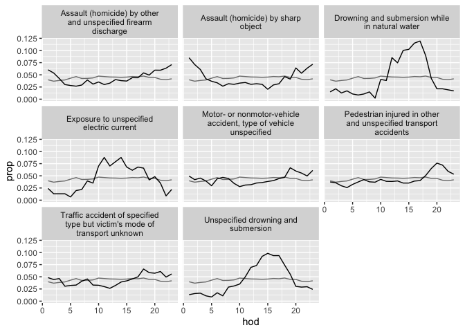
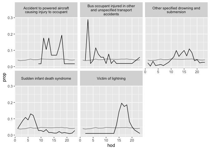
Table 16: A sample of four diseases and four hours from hod2 data frame.
| 4638 |
8 |
B16 |
4 |
| 4787 |
8 |
E84 |
3 |
| 4852 |
8 |
I21 |
2205 |
| 5028 |
8 |
N18 |
315 |
| 5305 |
9 |
B16 |
7 |
| 5473 |
9 |
E84 |
1 |
| 5536 |
9 |
I21 |
2209 |
| 5707 |
9 |
N18 |
333 |
| 5994 |
10 |
B16 |
10 |
| 6153 |
10 |
E84 |
7 |
| 6217 |
10 |
I21 |
2434 |
| 6392 |
10 |
N18 |
343 |
| 6689 |
11 |
B16 |
6 |
| 6856 |
11 |
E84 |
3 |
| 6915 |
11 |
I21 |
2128 |
a
|
| 4638 |
Acute hepatitis B |
| 4787 |
Cystic fibrosis |
| 4852 |
Acute myocardial infarction |
| 5028 |
Chronic renal failure |
| 5305 |
Acute hepatitis B |
| 5473 |
Cystic fibrosis |
| 5536 |
Acute myocardial infarction |
| 5707 |
Chronic renal failure |
| 5994 |
Acute hepatitis B |
| 6153 |
Cystic fibrosis |
| 6217 |
Acute myocardial infarction |
| 6392 |
Chronic renal failure |
| 6689 |
Acute hepatitis B |
| 6856 |
Cystic fibrosis |
| 6915 |
Acute myocardial infarction |
b
|
| 4638 |
0.0381 |
| 4787 |
0.0294 |
| 4852 |
0.0471 |
| 5028 |
0.0412 |
| 5305 |
0.0667 |
| 5473 |
0.0098 |
| 5536 |
0.0472 |
| 5707 |
0.0436 |
| 5994 |
0.0952 |
| 6153 |
0.0686 |
| 6217 |
0.0520 |
| 6392 |
0.0449 |
| 6689 |
0.0571 |
| 6856 |
0.0294 |
| 6915 |
0.0455 |
c
|
| 4638 |
21915 |
0.0427 |
| 4787 |
21915 |
0.0427 |
| 4852 |
21915 |
0.0427 |
| 5028 |
21915 |
0.0427 |
| 5305 |
22401 |
0.0436 |
| 5473 |
22401 |
0.0436 |
| 5536 |
22401 |
0.0436 |
| 5707 |
22401 |
0.0436 |
| 5994 |
24321 |
0.0474 |
| 6153 |
24321 |
0.0474 |
| 6217 |
24321 |
0.0474 |
| 6392 |
24321 |
0.0474 |
| 6689 |
23843 |
0.0465 |
| 6856 |
23843 |
0.0465 |
| 6915 |
23843 |
0.0465 |
d
|