6 Policy Evaluation I - Binary Treatment
Before you jump into this chapter, we recommend that you’ve read:
- Introduction to Machine Learning
- Introduction to Causal Inference
- ATE I - Binary treatment
- HTE I - Binary treatment
6.1 What is a policy?
- Definition: policy as a treatment rule
- Examples of policies:
- “Always treat” \(\pi(x) \equiv 1\)
- “Never treat” \(\pi(x) \equiv 0\)
In the next module you will also learn how to estimate policies from data.
6.2 Evaluating policies in experimental settings
set.seed(1)
n <- 1000
p <- 4
X <- matrix(runif(n*p), n, p)
W <- rbinom(n, prob = .5, size = 1)
Y <- .5*X[,2] + (X[,1] - .5)*W + .01 * rnorm(n)

y.norm <- (Y - min(Y))/(max(Y)-min(Y)) # just for plottingplot(X[,1], X[,2], pch=ifelse(W, 21, 23), cex=1.5, bg=gray(y.norm), xlab="X1", ylab="X2")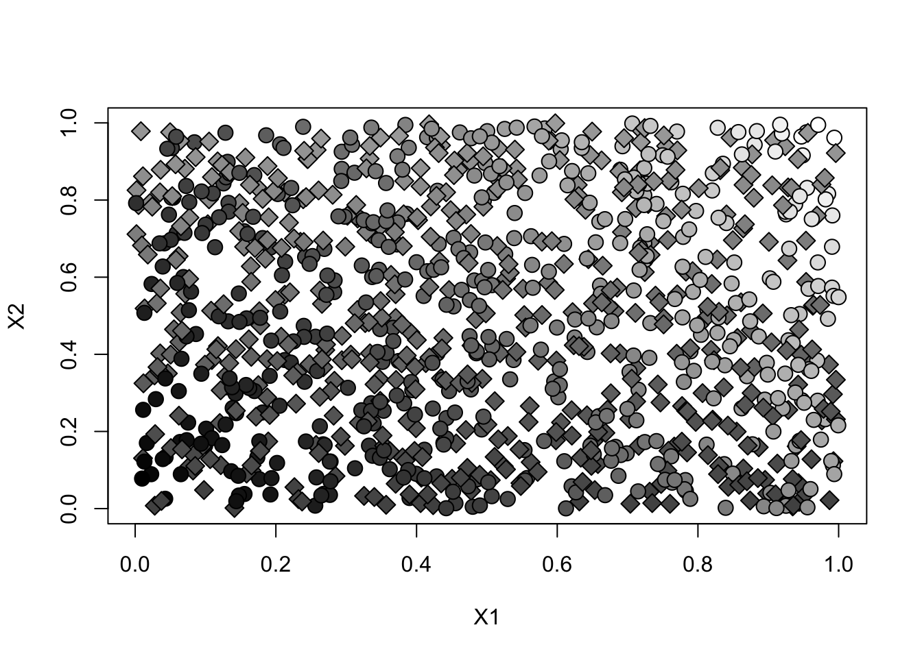
- Note how observations in the top right have higher outcome.
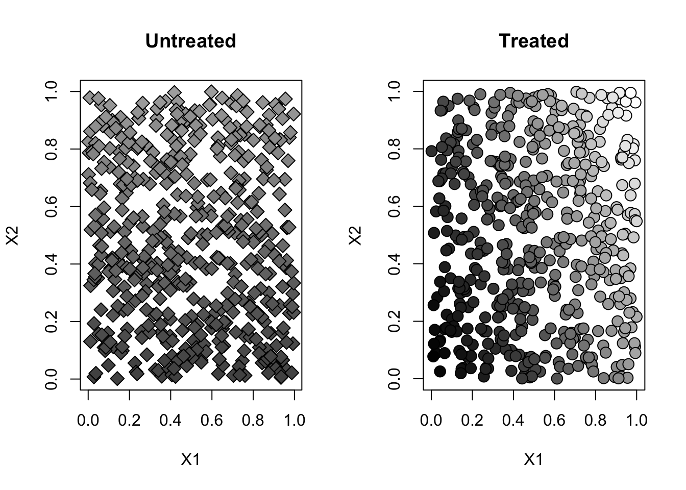
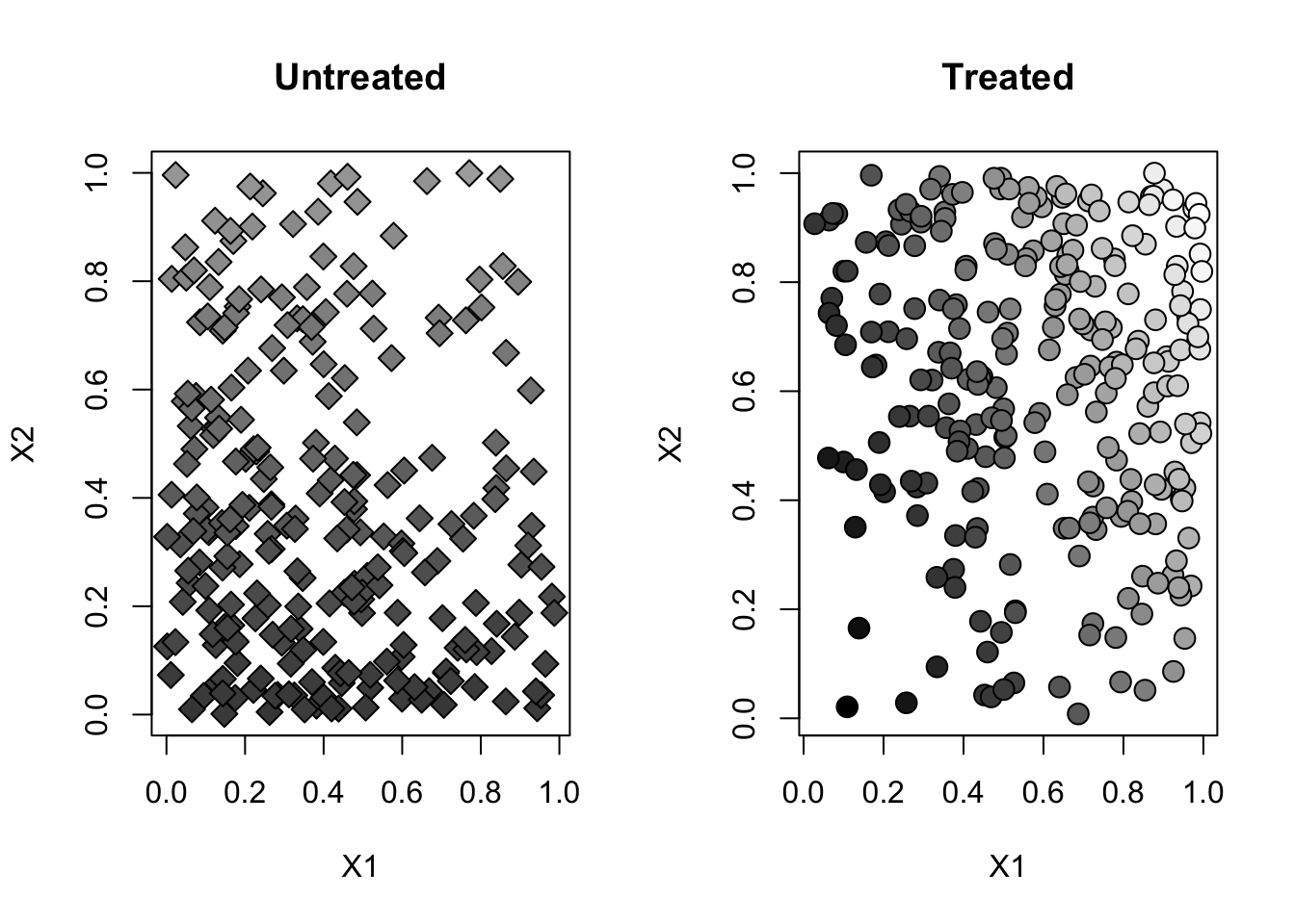
- Here’s a graph of each treated and untreated population separately.
par(mfrow=c(1,2))
for (w in c(0, 1)) {
  plot(X[W==w,1], X[W==w,2], pch=ifelse(W[W==w], 21, 23), cex=1.5,
       bg=gray(y.norm[W==w]), main=ifelse(w, "Treated", "Untreated"),
       xlab="X1", ylab="X2")
}
- Consider the following exogenously given policy (e.g. estimated on prior data) \[\begin{equation} \tag{6.1} \pi(x) = \begin{cases} 1 \qquad \text{if }x_1 > .5 \text{ and }x_2 > .5, \\ 0 \qquad \text{otherwise}. \end{cases} \end{equation}\]
Let’s evaluate the policy (6.1) in an experimental setting. This policy divides the plane into two regions.
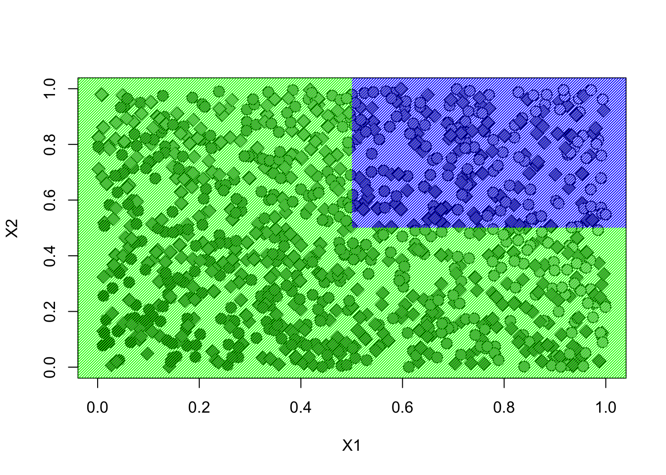
Let’s denote the region in blue by \(A = \{X_{i, 1} > .5, X_{i,2} > 5 \}\).
In the blue region, the policy \(\pi\) treats. In that region, its average outcome is the same as the average outcome for the treated population. \[\begin{align} \mathbb{E}[Y(\pi(X_i)) | A] = \mathbb{E}[Y(1)|A] = \mathbb{E}[Y|A, W=1] \end{align}\]
In the green region, the policy \(\pi\) does not treat. In that region, its average outcome is the same as the average outcome for the untreated population. \[\begin{align} \mathbb{E}[Y(\pi(X_i)) | A^c] = \mathbb{E}[Y(0)|A^c] = \mathbb{E}[Y|A^c, W=0] \end{align}\]
The final outcome will be an average of the two regions, weighted by the size of the each region.
\[\begin{align} \mathbb{E}[Y(\pi(X_i))] &= \mathbb{E}[Y(\pi(X_i)) | A] P(A) + \mathbb{E}[Y(\pi(X_i)) | A^c] P(A^c) \\ &= \mathbb{E}[Y | A, W=1] P(A) + \mathbb{E}[Y | A^c, W=0] P(A^c) \\ \end{align}\]
In an experimental setting, this suggests the following estimator.
# Only valid for experimental data!
A <- (X[,1] > .5) & (X[,2] > .5)
value.estimate <- mean(Y[A & (W==1)]) * mean(A) + mean(Y[!A & (W==0)]) * mean(!A)
value.stderr <- sqrt(var(Y[A & (W==1)]) / sum(A & (W==1)) * mean(A)^2 + var(Y[!A & (W==0)]) / sum(!A & W==0) * mean(!A)^2)
print(paste("Value estimate:", value.estimate, "Std. Error:", value.stderr))
## [1] "Value estimate: 0.307429588663063 Std. Error: 0.00638961774980037"Following a similar thought process to above, ee can also estimate the difference in value between two given policies. For example. let’s consider the gain from switching from a “never treat” policy to the policy \(\pi\).
In the green region, the policy \(\pi\) does not treat, and neither does the “never treat” policy. Therefore, the gain there is exactly zero.
In the blue region, the policy \(\pi\) treats, and the “never treat” policy does not. Therefore, the gain there is the average treatment effect in that region.
Putting these together, the expected difference in value equals the following. \[\begin{align} \mathbb{E}[Y(\pi(X_i))] - \mathbb{E}[Y(0)] &= \left( \mathbb{E}[Y(\pi(X_i)) | A] - \mathbb{E}[Y(0)] \right) P(A) + 0 P(A^c)\\ &= \left( \mathbb{E}[Y | A, W=1] - \mathbb{E}[Y | A, W=0] \right) P(A) \\ \end{align}\]
# Only valid for experimental data!
A <- (X[,1] > .5) & (X[,2] > .5)
diff.estimate <- (mean(Y[A & (W==1)]) - mean(Y[A & (W==0)])) * mean(A)
diff.stderr <- sqrt(var(Y[A & (W==1)]) / sum(A & (W==1)) + var(Y[A & (W==0)]) / sum(A & W==0)) * mean(A)^2
print(paste("Difference estimate:", diff.estimate, "Std. Error:", diff.stderr))
## [1] "Difference estimate: 0.063254241888017 Std. Error: 0.000861530592945719"6.3 Evaluating policies in observational settings
set.seed(1)
n <- 500
p <- 4
X <- matrix(runif(n*p), n, p)
e <- 1/(1+exp(-3*(X[,1]-.5)-3*(X[,2]-.5)))
W <- rbinom(n, prob = e, size = 1)
Y <- .5*X[,2] + (X[,1] - .5)*W + .01 * rnorm(n)

y.norm <- (Y - min(Y))/(max(Y)-min(Y)) # just for plottingplot(X[,1], X[,2], pch=ifelse(W, 21, 23), cex=1.5, bg=gray(y.norm), xlab="X1", ylab="X2")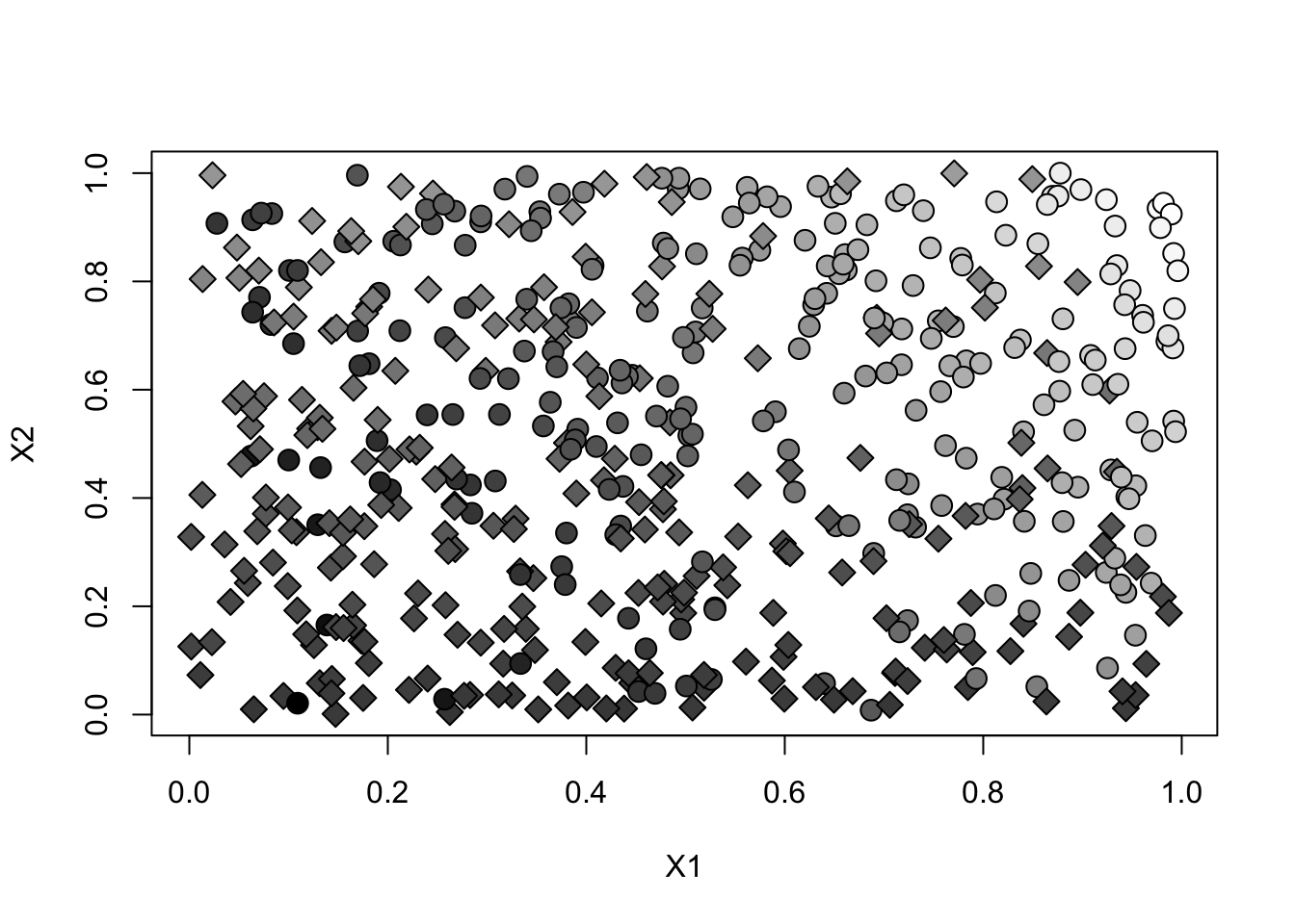
Note how in this setting treatment assignment isn’t independent from observed covariates. Individuals with high values of \(X_{i1}\) and \(X_{i2}\) are more likely to be treated and to have higher outcomes. This violates conditional unconfoundedness.
par(mfrow=c(1,2))
for (w in c(0, 1)) {
  plot(X[W==w,1], X[W==w,2], pch=ifelse(W[W==w], 21, 23), cex=1.5,
       bg=gray(y.norm[W==w]), main=ifelse(w, "Treated", "Untreated"),
       xlab="X1", ylab="X2")
}
If we “naively” used the estimators based on sample averages above, the policy value estimate would be biased. Would the bias be upward or downward?
Estimating the value of policy (6.1).
# Valid in observational and experimental settings
library(grf)

forest <- causal_forest(X, Y, W, num.trees=200)  # increae num.tree
tau.hat <- predict(forest)$predictions
mu.hat.1 <- forest$Y.hat + (1 - forest$W.hat) * tau.hat
mu.hat.0 <- forest$Y.hat - forest$W.hat * tau.hat
gamma.hat.1 <- mu.hat.1 + W/forest$W.hat * (Y - mu.hat.1)
gamma.hat.0 <- mu.hat.0 + (1-W)/(1-forest$W.hat) * (Y - mu.hat.0)

pi.scores <- ifelse((X[,1] > .5) & (X[,2] > .5), gamma.hat.1, gamma.hat.0)
value.estimate <- mean(pi.scores)
value.stderr <- sd(pi.scores) / sqrt(length(pi.scores))
print(paste("Value estimate:", value.estimate, "Std. Error:", value.stderr))
## [1] "Value estimate: 0.313117026575287 Std. Error: 0.0108119530358971"Estimating the difference between policy (6.1) and the “never treat” policy.
# Valid in observational and experimental settings
diff.scores <- pi.scores - gamma.hat.0
diff.estimate <- mean(diff.scores)
diff.stderr <- sd(diff.scores) / sqrt(length(diff.scores))
print(paste("diff estimate:", diff.estimate, "Std. Error:", diff.stderr))
## [1] "diff estimate: 0.0607159777263377 Std. Error: 0.00611108582515742"6.3.1 Aside: More complex policies
Policy (6.1) that was very easy to describe (“treat if \(X_1\) and \(X_2\) are both high”). But in fact the code and mathematical details above go through even if the policy is more complicated and high-dimensional. This will be the case with some policies that we’ll learn in the next section.