5 HTE I: Binary treatment
Before you jump into this tutorial, please make sure you’ve read:
5.1 Setup
data <- read.csv(file = "https://raw.githubusercontent.com/gsbDBI/ExperimentData/master/Welfare/ProcessedData/welfarenolabel3.csv")covariates <- c("income", "educ", "marital", "sex", "polviews")
outcome <- "y"
treatment <- "w"
data <- data[1:10000,] # for now
num.groups <- 5
n <- nrow(data)5.2 Pre-specified hypotheses
We are interested in testing whether pre-specified null hypotheses of the form \[\begin{equation} \tag{5.1} H_0: \mathbb{E}[Y(1) - Y(0) | G_{i}=1] = \mathbb{E}[Y(1) - Y(0) | G_{i}=0]. \end{equation}\]
That is, that the treatment effect is the same regardless of membership to some group \(G_i\). Importantly, for now we’ll assume that the group \(G_i\) was decided before running the experiment.
In experimental data, if the both the treatment \(W_i\) and group membership \(G_i\) are binary, we can write \[\begin{equation} \tag{5.2} \mathbb{E}[Y_i | W_i, G_i] = \beta_0 + \beta_w W_i + \beta_g G_i + \beta_{wg} X_i G_i. \end{equation}\]
This decomposition is true without loss of generality. Why?
This allows us to write the average effects of \(W_i\) and \(G_i\) on \(Y_i\) in the following way, \[\begin{equation} \tag{5.3} \begin{aligned} \mathbb{E}[Y(1) | G_i=1] &= \mathbb{E}[Y| W_i=1, G_i=1] = \beta_0 + \beta_w + \beta_g + \beta_{wg} \\ \mathbb{E}[Y(1) | G_i=0] &= \mathbb{E}[Y| W_i=1, G_i=0] = \beta_0 + \beta_w \\ \mathbb{E}[Y(0) | G_i=1] &= \mathbb{E}[Y| W_i=1, G_i=1] = \beta_0 + \ \ \ \ + \beta_g \\ \mathbb{E}[Y(0) | G_i=0] &= \mathbb{E}[Y| W_i=1, G_i=1] = \beta_0. \end{aligned} \end{equation}\]
Rewriting the null hypothesis (5.1) in terms of the decomposition (5.3), we see that it boils down to a test about the coefficient in the interaction: \(\beta_{xw} = 0\). Here’s an example:
# Example: suppose this group was defined prior to collecting the data.
data$conservative <- factor(data$polviews < 4)  # binary
group <- 'conservative'
# Only valid for experimental data!
fmla <- formula(paste(outcome, ' ~ ', treatment, '*', group))
ols <- lm(fmla, data=data)
coeftest(ols, vcov=vcovHC(ols, type='HC2'))##
## t test of coefficients:
##
## Estimate Std. Error t value Pr(>|t|)
## (Intercept) 0.441134 0.008446 52.230 < 2e-16 ***
## w -0.347980 0.009635 -36.115 < 2e-16 ***
## conservativeTRUE -0.121201 0.015928 -7.609 3.01e-14 ***
## w:conservativeTRUE 0.082977 0.017658 4.699 2.65e-06 ***
## ---
## Signif. codes: 0 '***' 0.001 '**' 0.01 '*' 0.05 '.' 0.1 ' ' 1Interpret the results above.
When there are many groups, we need to correct for the fact that we are testing for multiple hypotheses, or we will end up with many false positives. Here’s a null hypothesis that our \[\begin{equation} \tag{5.1} H_0: \mathbb{E}[Y(1) - Y(0) | G_{i}=g] = \mathbb{E}[Y(1) - Y(0) | G_{i}=1] \qquad \text{(for many values of }g\text{)}. \end{equation}\]
The Bonferroni correction is a very conservative method for dealing with multiple hypothesis testing.
# Example: these groups must be defined prior to collecting the data.
group <- 'polviews'
# Only valid for experimental data!
# Likely too conservative to be useful.
fmla <- formula(paste(outcome, ' ~ ', treatment, '*', 'factor(', group, ')'))
ols <- lm(fmla, data=data)
interact <- which(sapply(names(coef(ols)), function(x) grepl("w:", x)))
ols.res <- coeftest(ols, vcov=vcovHC(ols, type='HC2'))
unadj.p.value <- ols.res[interact, 4]
adj.p.value <- p.adjust(unadj.p.value, method='bonferroni')
data.frame(estimate=coef(ols)[interact],
std.err=ols.res[interact,2],
unadj.p.value, adj.p.value)## estimate std.err unadj.p.value adj.p.value
## w:factor(polviews)2 0.0144885 0.0504350 0.77391115 1.0000000
## w:factor(polviews)3 -0.0305790 0.0501349 0.54191895 1.0000000
## w:factor(polviews)4 -0.0851243 0.0470780 0.07061270 0.4942889
## w:factor(polviews)4.1220088 -0.0148913 0.0566752 0.79275065 1.0000000
## w:factor(polviews)5 -0.1335512 0.0496252 0.00713144 0.0499201
## w:factor(polviews)6 -0.0763852 0.0511340 0.13525321 0.9467724
## w:factor(polviews)7 -0.1558322 0.0720950 0.03068162 0.2147713Often the Bonferroni correction is likely to be too stringent for most purposes. Another option is to use the Romano-Wolf correction. The code below performs this correction.
# Computes adjusted p-values following the Romano-Wolf method.
# For a reference, see http://ftp.iza.org/dp12845.pdf page 8
#  t.orig: vector of t-statistics from original model
#  t.boot: matrix of t-statistics from bootstrapped models
romano_wolf_correction <- function(t.orig, t.boot) {
  abs.t.orig <- abs(t.orig)
  abs.t.boot <- abs(t.boot)
  abs.t.sorted <- sort(abs.t.orig, decreasing = TRUE)

  max.order <- order(abs.t.orig, decreasing = TRUE)
  rev.order <- order(max.order)

  M <- nrow(t.boot)
  S <- ncol(t.boot)

  p.adj <- rep(0, S)
  p.adj[1] <- mean(apply(abs.t.boot, 1, max) > abs.t.sorted[1])
  for (s in seq(2, S)) {
    cur.index <- max.order[s:S]
    p.init <- mean(apply(abs.t.boot[, cur.index, drop=FALSE], 1, max) > abs.t.sorted[s])
    p.adj[s] <- max(p.init, p.adj[s-1])
  }
  p.adj[rev.order]
}

# Computes adjusted p-values for linear regression (lm) models.
summary_rw_lm <- function(model, indices=NULL, cov.type="HC2", num.boot=10000, seed=2020) {

  if (is.null(indices)) {
    indices <- 1:nrow(coef(summary(model)))
  }
  # Grab the original t values.
  summary <- coef(summary(model))[indices,,drop=FALSE]
  t.orig <- summary[, "t value"]

  # Null resampling.
  # This is a bit of trick to speed up bootstrapping linear models.
  # Here, we don't really need to re-fit linear regressions, which would be a bit slow.
  # We know that betahat ~ N(beta, Sigma), and we have an estimate Sigmahat.
  # So we can approximate "null t-values" by
  #  - Draw beta.boot ~ N(0, Sigma-hat)     note the 0 here, this is what makes it a *null* t-value.
  #  - Compute t.boot = beta.boot / sqrt(diag(Sigma.hat))
  Sigma.hat <- sandwich::vcovHC(model, type=cov.type)[indices, indices]
  se.orig <- sqrt(diag(Sigma.hat))
  num.coef <- length(se.orig)
  beta.boot <- MASS::mvrnorm(n=num.boot, mu=rep(0, num.coef), Sigma=Sigma.hat)
  t.boot <- sweep(beta.boot, 2, se.orig, "/")
  p.adj <- romano_wolf_correction(t.orig, t.boot)

  result <- cbind(summary[,c(1,2,4),drop=F], p.adj)
  colnames(result) <- c('Estimate', 'Std. Error', 'Orig. p-value', 'Adj. p-value')
  result
}
# Only valid for experimental data!
fmla <- formula(paste(outcome, ' ~ ', treatment, '*', 'factor(', group, ')'))
ols <- lm(fmla, data=data)
interact <- which(sapply(names(coef(ols)), function(x) grepl("w:", x)))
summary_rw_lm(ols, indices=interact)## Estimate Std. Error Orig. p-value Adj. p-value
## w:factor(polviews)2 0.0144885 0.0560185 0.7959202 0.9412
## w:factor(polviews)3 -0.0305790 0.0553014 0.5803085 0.8479
## w:factor(polviews)4 -0.0851243 0.0524521 0.1046434 0.2484
## w:factor(polviews)4.1220088 -0.0148913 0.0613334 0.8081713 0.9412
## w:factor(polviews)5 -0.1335512 0.0543942 0.0140957 0.0556
## w:factor(polviews)6 -0.0763852 0.0549884 0.1648285 0.3417
## w:factor(polviews)7 -0.1558322 0.0705879 0.0272926 0.0935When working with either experimental or observational data, one can use AIPW scores \(\widehat{\Gamma}_i\) in place of the raw outcomes \(Y_i\). Here’s how to do it using GRF.
# Valid for both experimental and observational data.
cf <- causal_forest(X=data[,covariates],
                    Y=data[,outcome],
                    W=data[,treatment],
                    W.hat=NULL, # use true propensity score if known
                    num.trees=200)  # in practice use num.trees ~ nrow(data)
fmla <- formula(paste('scores ~ ', treatment, '* factor(', group, ')'))
ols <- lm(fmla, data=transform(data, scores=get_scores(cf)))
interact <- which(sapply(names(coef(ols)), function(x) grepl("w:", x)))
summary_rw_lm(ols, indices=interact)
## Estimate Std. Error Orig. p-value Adj. p-value
## w:factor(polviews)2 -0.00792069 0.122445 0.948424 0.9999
## w:factor(polviews)3 -0.00971677 0.120877 0.935932 0.9999
## w:factor(polviews)4 0.01698675 0.114650 0.882218 0.9999
## w:factor(polviews)4.1220088 -0.02304272 0.134062 0.863535 0.9999
## w:factor(polviews)5 0.01035451 0.118895 0.930602 0.9999
## w:factor(polviews)6 -0.01676302 0.120193 0.889084 0.9999
## w:factor(polviews)7 0.20342214 0.154291 0.187389 0.4891One can also construct AIPW scores using any other method. In ATE I we showed how to construct AIPW scores using Lasso and splines via glmnet and splines.
5.3 Data-driven hypotheses
Instead of coming up with hypotheses before running the experiment…
5.3.1 Via causal trees
When dealing with observational data, we can use the honest.causalTree function from the causalTree package.
# Only valid for experimental data!

# remotes::install_github('susanathey/causalTree') # Uncomment this to install the causalTree package
library(causalTree)

fmla <- paste(outcome, " ~", paste(covariates, collapse = " + "))

# Dividing data into three subsets
indices <- split(seq(nrow(data)), sort(seq(nrow(data)) %% 3))
names(indices) <- c('split', 'est', 'test')

# Fitting the forest
ct.unpruned <- honest.causalTree(
  formula=fmla,            # Define the model
  data=data[indices$split,],
  treatment=data[indices$split, treatment],
  est_data=data[indices$est,],
  est_treatment=data[indices$est, treatment],
  minsize=2,                 # Min. number of treatment and control cases in each leaf
  HonestSampleSize=length(indices$est), #  Num obs used in estimation after splitting
  # Recommended parameters.
  split.Rule="CT",            # Define the splitting option
  cv.option="TOT",            # Cross validation options
  cp=0,                       # Complexity parameter
  split.Honest=TRUE,          # Use honesty when splitting
  cv.Honest=TRUE             # Use honesty when performing cross-validation
)

# Table of cross-validated values by tuning parameter.
ct.cptable <- as.data.frame(ct.unpruned$cptable)

# Obtain optimal complexity parameter to prune tree.
cp.selected <- which.min(ct.cptable$xerror)
cp.optimal <- ct.cptable[cp.selected, "CP"]

# Prune the tree at optimal complexity parameter.
ct.pruned <- prune(tree=ct.unpruned, cp=cp.optimal)

# Predict point estimates (on estimation sample)
tau.hat.est <- predict(ct.pruned, newdata=data[indices$est,])

# Create a factor column 'leaf' indicating leaf assignment in the estimation set
num.leaves <- length(unique(tau.hat.est))
leaf <- factor(tau.hat.est, levels=sort(unique(tau.hat.est)), labels = seq(num.leaves))
Note: if your tree is not splitting at all, try decreasing the parameter minsize that controls the minimum size of each leaf. For more details, please refer to the package documentation.
rpart.plot(
  x=ct.pruned,        # Pruned tree
  type=3,             # Draw separate split labels for the left and right directions
  fallen=TRUE,        # Position the leaf nodes at the bottom of the graph
  leaf.round=1,       # Rounding of the corners of the leaf node boxes
  extra=100,          # Display the percentage of observations in the node
  branch=.1,          # Shape of the branch lines
  box.palette="RdBu") # Palette for coloring the node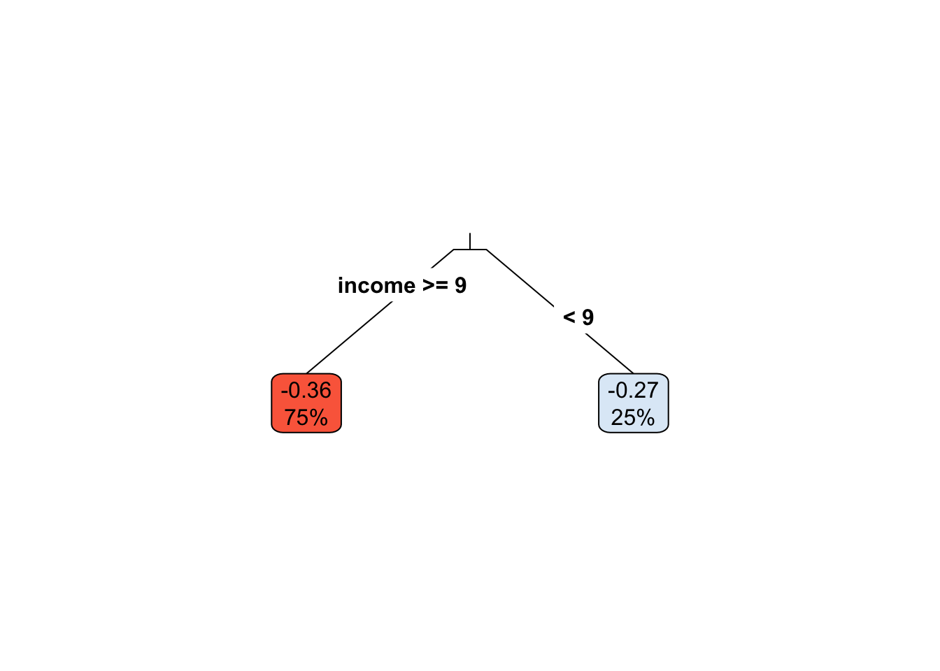
Following the same logic as above, we can test if the average treatment effect within each leaf is different from the leaf with smallest (or most negative) tratment effect. This is valid because of our careful sample-splitting scheme.
# Only for experimental data!
fmla <- paste0(outcome, ' ~ ', treatment, '*leaf')
ols <- lm(fmla, data=transform(data[indices$est,], leaf=leaf))
interact <- which(sapply(names(coef(ols)), function(x) grepl("w:", x)))
if (num.leaves > 2) {
  # Use Romano-Wolf test correction if there are three or more leaves
  summary_rw_lm(ols, indices=interact, cov.type = 'HC2')
} else if (num.leaves == 2) {
  # Case of exactly two leaves
  coeftest(ols, vcov=vcovHC(ols, 'HC2'))[interact,,drop=F]
} else {
  print("Skipping since there's a single leaf.")
}
## Estimate Std. Error t value Pr(>|t|)
## w:leaf2 0.0894818 0.0296649 3.01642 0.002577165.3.2 Via grf
Assessing systematic variation in treatment effect heterogeneity is a difficult task. Let’s begin by looking at some popular measures and see how they may lead to subtle pitfalls.
First, having fit a non-parametric method such as a causal forest, a researcher may (incorrectly) start by looking at the distribution of its predictions of the treatment effect. One might be tempted to think: “if the histogram is concentrated at a point, then there is no heterogeneity; if the histogram is spread out, then our estimator has found interesting heterogeneity.” However, both of these assertions may be false!
If the histogram is concentrated at a point, we may simply be underpowered: our method was not able to detect any heterogeneity, but maybe it would detect it if we had more data. If the histogram is spread out, we may be simply overfitting: our model is producing very noisy estimates \(\widehat{\tau}(X_i)\), but in fact the truth \(\tau_i\) could be a lot smoother.
# Do not use!
X <- data[,covariates]
W <- data[[treatment]]
Y <- data[[outcome]]

cf <- causal_forest(X, Y, W, num.trees=200)
tau.hat <- predict(cf)$predictions
hist(tau.hat, main="CATE estimates", freq=F)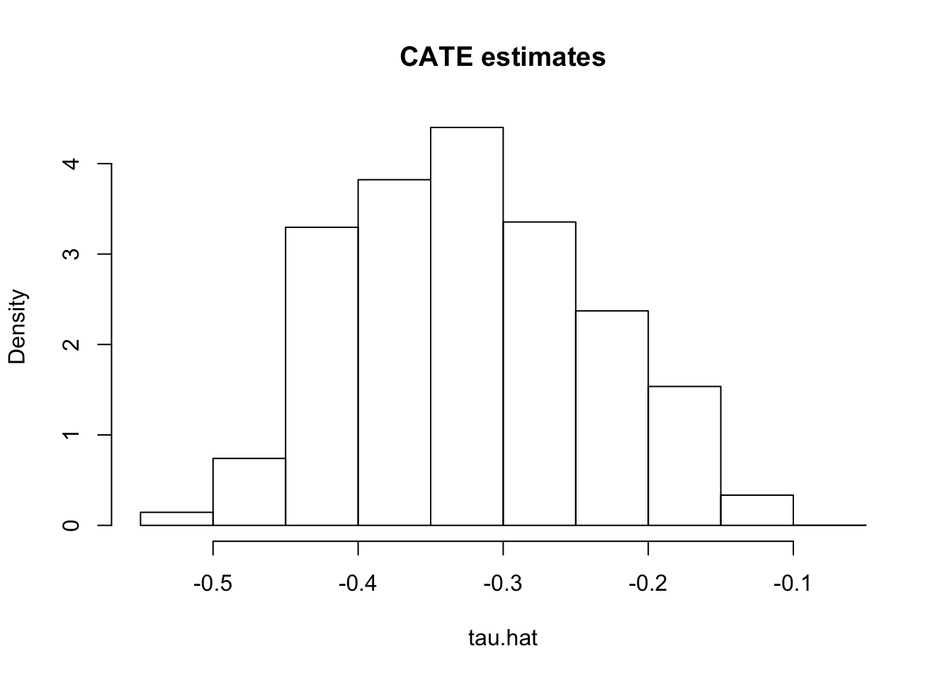
Next, the grf package also produces a measure of variable importance that indicates how often a variable was used in a tree split. Again, much like the histogram aboove, this can be a rough diagnostic, but it should not be interpreted as indicating that, for example, variable with low importance is not related to heterogeneity. The reasoning is the same as the one presented in the causal trees section: if two covariates are highly correlated, the trees might split on one covariate but not the other. However, if one was removed, the trees might split on the one remaining, and the leaf definitions might be unchanged.
var_imp <- c(variable_importance(cf))
names(var_imp) <- covariates
sorted_var_imp <- sort(var_imp, decreasing = TRUE)
sorted_var_imp[1:5]
## income polviews marital educ sex
## 0.4967509 0.1616885 0.1574553 0.1483933 0.03571215.3.2.1 Finding subgroups via grf
# Valid for both observational and experimental data!

X <- data[,covariates]
W <- data[[treatment]]
Y <- data[[outcome]]

n.folds <- 5
indices <- split(seq(n), sort(seq(n) %% n.folds))

res <- lapply(indices, function(idx) {

  forest.m <- regression_forest(X[-idx,], Y[-idx], num.trees=200)  # increase num.trees
  forest.e <- regression_forest(X[-idx,], W[-idx], num.trees=200)  # increase num.trees

  m.hat <- predict(forest.m, X[idx,])$predictions
  e.hat <- predict(forest.e, X[idx,])$predictions

  forest.tau <- causal_forest(X[-idx,], Y[-idx], W[-idx], num.trees=200)  # increase num.trees
  tau.hat <- predict(forest.tau, X[idx,])$predictions

  mu.hat.0 <- m.hat - e.hat * tau.hat
  mu.hat.1 <- m.hat + (1 - e.hat) * tau.hat

  aipw.scores <- (mu.hat.1 - mu.hat.0
                + W[idx] / e.hat * (Y[idx] -  mu.hat.1)
                - (1 - W[idx]) / (1 - e.hat) * (Y[idx] -  mu.hat.0))

  tau.hat.quantiles <- quantile(tau.hat, probs=seq(0, 1, length.out=num.groups+1))
  ranking <- cut(tau.hat, tau.hat.quantiles, include.lowest = TRUE,
                 labels = paste0("Q", seq(num.groups)))

  data.frame(aipw.scores, tau.hat, ranking=factor(ranking))
})
res <- do.call(rbind, res)
Having run the code above we can test, e.g., if the prediction within each group is larger than the one in the first group.
ols <- lm(aipw.scores ~ ranking, data=res)
coeftest(ols, vcov=vcovHC(ols, type='HC2'))
##
## t test of coefficients:
##
## Estimate Std. Error t value Pr(>|t|)
## (Intercept) -0.38157 0.01964 -19.431 < 2e-16 ***
## rankingQ2 0.01162 0.02754 0.422 0.6730
## rankingQ3 0.04652 0.02745 1.694 0.0902 .
## rankingQ4 0.06669 0.02702 2.469 0.0136 *
## rankingQ5 0.16100 0.02567 6.272 3.7e-10 ***
## ---
## Signif. codes: 0 '***' 0.001 '**' 0.01 '*' 0.05 '.' 0.1 ' ' 1And as before we may want to use correct for multiple hypothesis testing using the same methods as above.
interact <- which(sapply(names(coef(ols)), function(x) grepl("Q", x)))
summary_rw_lm(ols, indices=interact)
## Estimate Std. Error Orig. p-value Adj. p-value
## rankingQ2 0.0116239 0.0264047 6.59786e-01 0.6623
## rankingQ3 0.0465169 0.0263482 7.75158e-02 0.1346
## rankingQ4 0.0666940 0.0263714 1.14531e-02 0.0291
## rankingQ5 0.1609990 0.0263780 1.07604e-09 0.0000We can also check if different groups have different average covariate levels across n-tiles of estimated conditional treatment effects. Recalling the warning against using variable importance measures, it is possible that one covariate is not “important” in splitting, but yet it varies strongly with treatment effects. The approach of comparing all covariates across n-tiles of treatment effects presents a fuller picture of how high-treatment-effect individuals differ fom low-treatment-effect individuals.
mapply(function(covariate) {
      fmla <- formula(paste0(covariate, "~ 0 + ranking"))
      ols.x <- lm(fmla, data=transform(data, ranking=res$ranking))
      t(coef(summary(ols.x))[,1:2])
}, covariates[1:3], SIMPLIFY = F)  # Showing only first three
## $income
## rankingQ1 rankingQ2 rankingQ3 rankingQ4 rankingQ5
## Estimate 10.10907 -47.73729 -104.15519 -135.99099 -139.01554
## Std. Error 6.38224 6.43024 6.40291 6.41412 6.41734
##
## $educ
## rankingQ1 rankingQ2 rankingQ3 rankingQ4 rankingQ5
## Estimate 12.61775 11.85606 10.56587 8.94492 2.98897
## Std. Error 1.27211 1.28168 1.27623 1.27846 1.27910
##
## $marital
## rankingQ1 rankingQ2 rankingQ3 rankingQ4 rankingQ5
## Estimate 1.75310 1.920483 0.437126 2.322984 3.305263
## Std. Error 0.38724 0.390152 0.388494 0.389174 0.3893695.3.2.2 Partial dependence plots
5.3.2.3 Best linear projection
This function provides a (doubly robust) fit to the linear model \(\widehat{tau}(Xi) = \beta_0 + A_i' \beta_1\), where \(A_i\) could be a subset of the covariate columns.
grf::best_linear_projection(cf, X[,1:2])##
## Best linear projection of the conditional average treatment effect.
## Confidence intervals are cluster- and heteroskedasticity-robust (HC3):
##
## Estimate Std. Error t value Pr(>|t|)
## (Intercept) -3.219e-01 9.029e-03 -35.649 <2e-16 ***
## income -2.008e-05 2.898e-05 -0.693 0.488
## educ -1.934e-04 1.605e-04 -1.205 0.228
## ---
## Signif. codes: 0 '***' 0.001 '**' 0.01 '*' 0.05 '.' 0.1 ' ' 15.3.2.4 Assessing heterogeneity
test_calibration(cf)##
## Best linear fit using forest predictions (on held-out data)
## as well as the mean forest prediction as regressors, along
## with one-sided heteroskedasticity-robust (HC3) SEs:
##
## Estimate Std. Error t value Pr(>t)
## mean.forest.prediction 0.9979 0.0246 40.564 < 2e-16 ***
## differential.forest.prediction 0.6928 0.0918 7.547 2.42e-14 ***
## ---
## Signif. codes: 0 '***' 0.001 '**' 0.01 '*' 0.05 '.' 0.1 ' ' 1