2 Introduction to Machine Learning

Click here for the Rmarkdown source: here

In this chapter, we’ll briefly introduce machine learning concepts that will be relevant later. We’ll focus in particular on problem of prediction, that is, to model some output variable from observed input covariates.

As with all the chapters in this tutorial, if you’d like to run this code on a different dataset, you can replace the toy dataset below with another data.frame of your choice. You might need to make a few minor changes to the code below; read the comments carefully.

library(grf)
library(rpart)
library(glmnet)
library(splines)
library(MASS)

set.seed(1)
n <- 2000
p <- 20
x <- mvrnorm(n, mu = rep(0, p), Sigma = toeplitz(.8^seq(p)))
y <- pmax(x[,1], 0) + sin(x[,2])*3 + x[,3]*x[,4] + sqrt(abs(x[,5])) + sqrt(p) * rnorm(n)
data <- data.frame(x=x, y=y)

n <- nrow(data)
outcome <- "y"
covariates <- paste0("x.", seq(p))

2.1 Key concepts

The prediction problem is to accurately guess the value of an some output variable, \(Y_i\) from input variables \(X_i\). For example, we might want to predict “house prices given house characteristics such as number of rooms, age of the building, and so on. The relationship between input and output is modeled in very general terms by some function \(f\) such that \[\begin{equation} \tag{2.1} Y_i = f(X_i) + \epsilon_i, \end{equation}\] where \(\epsilon_i\) represents all the errors that are not captured by information obtained from \(X_i\) via the mapping \(f\). We say that the error \(\epsilon_i\) is”irreducible".

We highlight that (2.1) is not causal. For an extreme example, consider taking \(Y_i\) to be “distance from equator” and \(X_i\) to be “average temperature.” We can still think of the problem of guessing (“predicting”) “distance from equator” given some information about “average temperature,” even though one would expect the former to cause the latter.

In general, we can’t know the “ground truth” \(f\), so we will approximate it from data. Given \(n\) data points \(\{(X_1, Y_1)\), \(\cdots\), \((X_n, Y_n)\}\), our goal is to obtain an estimated model \(\hat{f}\) such that our predictions \(\hat{Y}_i := \hat{f}(X_i)\) are “close” to the true outcome values \(Y_i\) given some criterion. To formalize this, we’ll follow these three steps:

Modeling: Decide on some suitable class of functions that our estimated model may belong to. In machine learning applications the class of functions can be very large and complex (e.g., deep decision trees, forests, high-dimensional linear models, etc). Also, we must decide on a loss function that serves as our criterion to evaluate the quality of our predictions (e.g., mean-squared error).
Fitting: Find the “best” fitting \(\hat{f}\) in the class of functions (e.g., the tree that minimizes the squared deviation between \(\hat{f}(X_i)\) and \(Y_i\) in our data).
Evaluation: Evaluate our fitted model \(\hat{f}\). That is, if we were given a new, yet unseen, input and output pair \((X',Y')\), we’d like to know if \(Y' \approx \hat{f}(X')\) by some metric.

For concreteness, let’s work through an example. Let’s say that, given the data simulated above, we’d like to predict \(Y_i\) from the first covariate \(X_{i1}\) only. Also, let’s say that our model class will be polynomials of degree \(q\) in \(X_{i1}\), and we’ll evaluate fit based on mean squared error. That is, \(\hat{f}(X_{i1}) = \hat{b}_0 + X_{i1}\hat{b}_{1} + X_{i1}^2 \hat{b}_2 + \cdots + X_{i1}^{q} \hat{b}_{q}\), where the coefficients are obtained by solving the following problem: \[\begin{equation} \hat{b} = \arg\min_{b} \sum_{i=1}^{m} \left( Y_i - b_0 + X_{i1}b_{1} + X_{i1}^2 b_2 + \cdots + X_{i1}^{q} b_{q} \right)^2. \end{equation}\]

An important question is what is \(q\), the degree of the polynomial. It controls the complexity of the model. One may imagine that more complex models are better, but that is not always true, because a very flexible model may try to simply interpolate over the data at hand, but fail to generalize well for new data points. We call this overfitting. To illustrate, in the figure below we let the degree be \(q=10\) but use only the first \(m=40\) data points. The fitted model is shown in green, and the original data points are in red.

# Note: this code assumes that the first covariate is continuous

# Fitting a flexible model on very little data
subset <- 1:40  # only a few data points
fmla <- formula(paste0(outcome, "~ poly(", covariates[1], ", 10)")) # high order poly
ols <- lm(fmla, data, subset=subset)

# Predicting on a grid of X1 values and plotting
x.grid <- seq(min(data[,covariates[1]]), max(data[,covariates[1]]), length.out=1000)
new.data <- data.frame(x.grid)
colnames(new.data) <- covariates[1]
y.hat <- predict(ols, newdata = new.data)

plot(data[subset, covariates[1]], data[subset, outcome], pch=21, bg="red", xlab="X1", ylab="Outcome", main="Example of overfitting")
lines(x.grid, y.hat, col="green", lwd=2)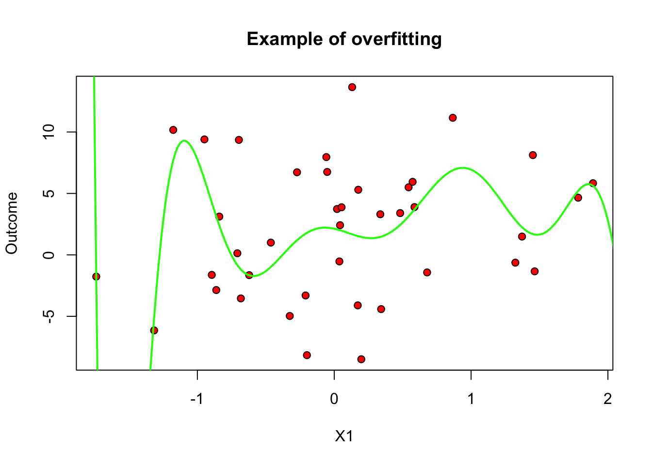

On the other hand, when \(q\) is too small relative to our data, we permit only very simple models and may suffer from misspecification bias. We call this underfitting. In the figure below we only allow for \(q=0\) (i.e., we’re fitting only constants).

# Note: this code assumes that the first covariate is continuous

# Fitting a constant model on very little data
subset <- 1:40  # only a few data points
fmla <- formula(paste0(outcome, "~ 1")) 
ols <- lm(fmla, data, subset=subset)

# Predicting on a grid of X1 values and plotting
x.grid <- seq(min(data[,covariates[1]]), max(data[,covariates[1]]), length.out=1000)
new.data <- data.frame(x.grid)
colnames(new.data) <- covariates[1]
y.hat <- predict(ols, newdata = new.data)

plot(data[subset, covariates[1]], data[subset, outcome], pch=21, bg="red", xlab="X1", ylab="Outcome", main="Example of underfitting")
lines(x.grid, y.hat, col="green", lwd=2)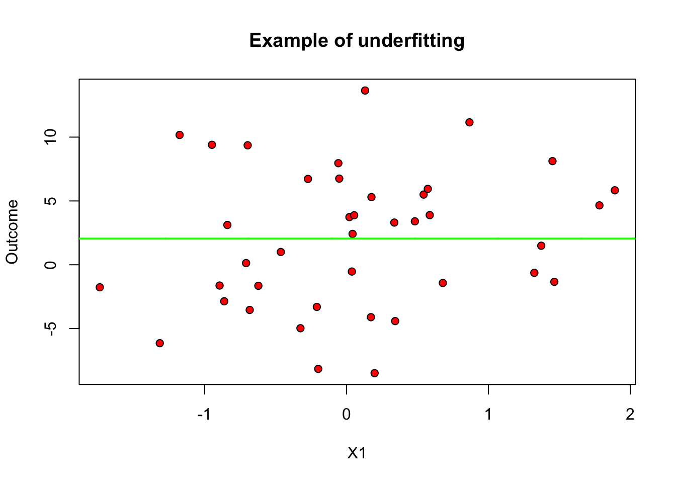

This tension is called the bias-variance trade-off: simpler models underfit and have more bias, more complex models overfit and have more variance.

One data-driven way of decide on appropriate level of complexity is to divide the available data into a training set (where the model is fit) and the validation set (where the model is evaluated). The next snippet of code uses the first half of the data to fit a polynomial of order \(q\), and then evaluates that polynomial on the second half.

poly.degree <- seq(8)
mse.estimates <- sapply(poly.degree, function(q) {
  # fitting on the training subset
  train <- 1:(n/2) 
  fmla <- formula(paste0(outcome, "~ poly(", covariates[1], ",", q,")"))
  ols <- lm(fmla, data=data, subset=train)
  
  # predicting on the validation subset
  y.hat <- predict(ols, newdata=data[-train,]) 
  squared.error <- (y.hat - data[-train, outcome])^2
  mse <- mean(squared.error)
  })

plot(poly.degree, mse.estimates, main="MSE estimates (train-test split)", ylab="log(MSE estimate)", xlab="Polynomial degree")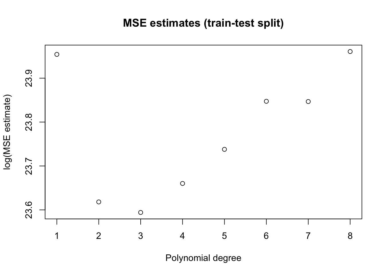

To make better use of the data we will often divide the data into \(K\) subsets, or folds. Then one fits \(K\) models, each using using \(K-1\) folds and then evaluation the fitted model on the remaining fold. This is called k-fold cross-validation.

n.folds <- 5 # K
poly.degree <- seq(8)

# Fold indices
indices <- split(seq(n), sort(seq(n) %% n.folds)) 

# Looping over polynomial degrees
mse.estimates <- sapply(seq(8), function(q) {
    fmla <- formula(paste0(outcome, "~ poly(", covariates[1], ",", q,")"))
    
    # Looping over folds 
    y.hat <- sapply(indices, function(fold.idx) {
        # Fit on K-1 folds
        ols <- lm(fmla, data=data[-fold.idx,])
        # Predict on Kth fold (left-out)
        predict(ols, newdata=data[fold.idx,])
    })
    squared.error <- (y.hat - data[, outcome])^2
    mean(squared.error)
})

  
plot(poly.degree, mse.estimates, main="MSE estimates (K-fold cross-validation)", ylab="MSE estimate", xlab="Polynomial degree")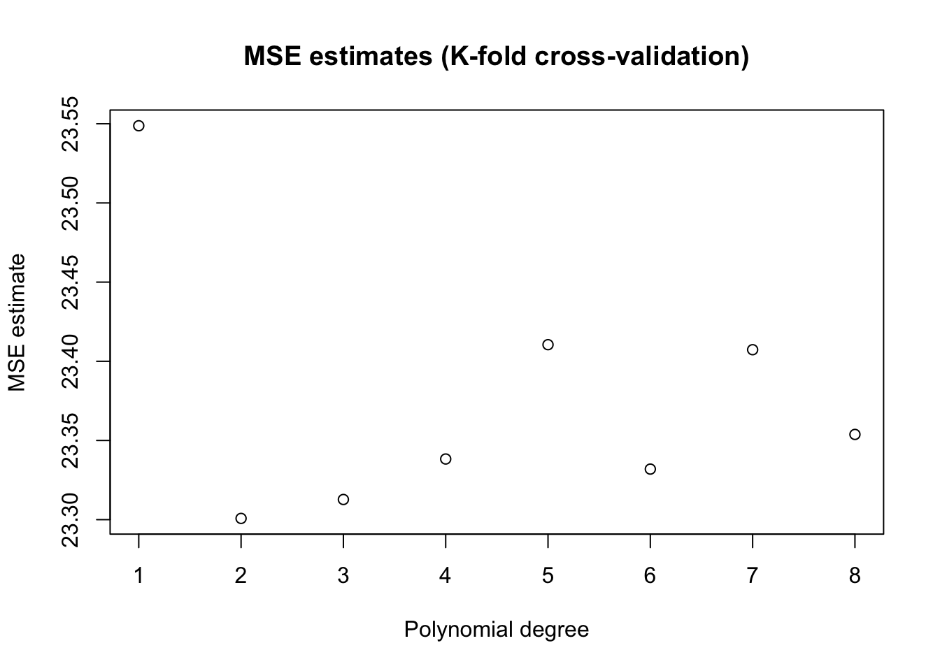

A final remark is that, in machine learning applications, the complexity of the model often is allowed to increase with the available data. In the example above, even though we weren’t very successful when fitting a high-dimensional model on very little data in the example above, if we had much more data perhaps such a model would be appropriate. The next figure again fits a 10th-order polynomial, but this time on many data points. Note how, at least in data-rich regions, the model is much better behaved (though it may still not be optimal). This is one of the benefits of using machine-learning based models: more data implies more flexible modeling, and therefore potentially better predictive power, provided that we are careful to avoid overfitting.

# Note: this code assumes that the first covariate is continuous

# Fitting a flexible model on very little data
subset <- 1:n  # now using much more data
fmla <- formula(paste0(outcome, "~ poly(", covariates[1], ", 10)")) # high order poly
ols <- lm(fmla, data, subset=subset)

# Predicting on a grid of X1 values and plotting
x.grid <- seq(min(data[,covariates[1]]), max(data[,covariates[1]]), length.out=1000)
new.data <- data.frame(x.grid)
colnames(new.data) <- covariates[1]
y.hat <- predict(ols, newdata = new.data)

plot(data[subset, covariates[1]], data[subset, outcome], pch=21, bg="red", xlab="X1", ylab="Outcome")
lines(x.grid, y.hat, col="green", lwd=2)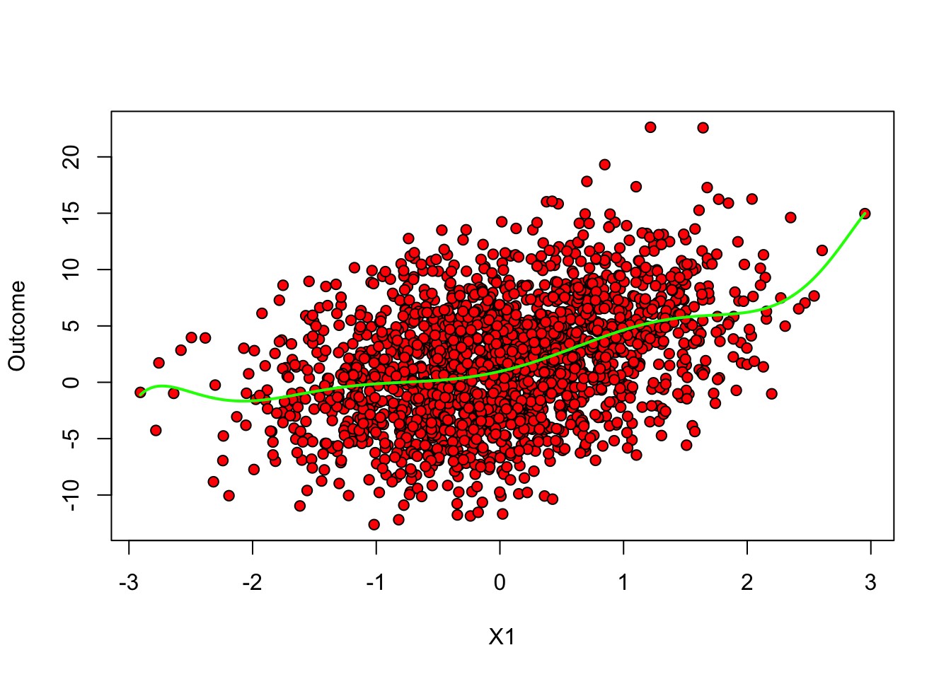

The example above based on polynomial regression was used mostly for illustration. In practice, there are often better performing algorithms. We’ll see some of them next.

Note on intepreting models A recurring theme below is that we will caution against interpreting the fitted model \(\hat{f}\) as evidence about aspects of the underlying data-generating process. In particular, we won’t be making any causal claims about the data in this chapter – but please hang tight, as estimating causal will be the one of the main topics presented in the next chapters.

2.2 Common machine learning algorithms

Next we’ll introduce three machine learning algorithms: trees, forests and regularized linear models. This is not an exhaustive list, but it they are common enough that every machine learning practitioner should know about them, and they have convenient R packages that allow for easy coding.

2.2.1 Decision trees

This class of algorithms divides the covariate space into regions, and estimates a constant prediction within each region.

In order to estimate a decision tree, we following a recursive partition algorithm. At each stage, we select one variable \(j\) and one split point \(s\), and divide the observations into “left” and “right” subsets, depending on whether \(X_{ij} \leq s\) or \(X_{ij} > s\). For regression problems, the variable and split points are often selected so that the sum of the variances of the outcome variable in each “child” subset is smallest. For classification problems, we split so as to separate the classes. Then, for each child, we separately repeat the process of finding variables and split points. This continues until a minimum subset size is reached, or improvement falls below some threshold.

At prediction time, to find the predictions for some point \(x\), we just follow the tree we just built, going left or right according to the selected variables and split points, until we reach a terminal node. Then, for regression problems, the predicted value at some point \(x\) is the average outcome of the observations in the same partition as the point \(x\). For classification problems, we output the majority class in the node.

Let’s estimate a decision tree using the R package rpart; see this tutorial for more information about it.

# Fit tree without pruning first
fmla <- formula(paste(outcome, "~", paste(covariates, collapse=" + ")))
tree <- rpart(fmla, data=data, cp=0, method="anova")  # use method="class" for classification

At this point, the fitted tree is likely much too deep, and probably overfits. Here’s a plot of what we have so far (without bothering to label the splits to avoid clutter).

plot(tree, uniform=TRUE)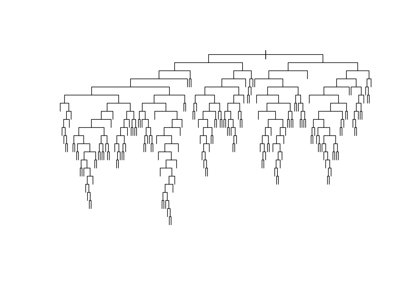

To reduce the complexity of the tree, we prune the tree: we collapse its leaves, permiting bias to increase but forcing variance to decrease, until the desired trade-off is achieved. In rpart, this is done by consider a modified loss function that takes into account the number of terminal nodes (i.e., the number of regions in which the original data was partitioned). Somewhat heuristically, if we denote a tree by \(T\) and its number of terminal nodes by \(|T|\), the modified regression problem can be written as: \[\begin{align} \tag{2.2} \widehat{T} = \min_{T} \sum_{i=1}^m \left( T(X_i) - Y_i \right)^2 + c_p |T|, \end{align}\] The complexity of the tree is controlled by the scalar parameter \(c_p\), denoted as cp in rpart. For each \(c_p\), we find the subtree \(\hat{T}\) that minimizes the loss above. Large values of \(c_p\) is lead to aggressively pruned trees, which have more bias and less variance. Small values of \(c_p\) allow for deeper trees whose predictions can vary more wildly. The plot below shows the cross-validated error (relative to a tree with only one node, which correspods to predicting the sample mean everywhere) for trees obtained at different levels of \(c_p\). The bias-variance trade-off is optimized at the point at which the cross-validated error is minimized.

plotcp(tree)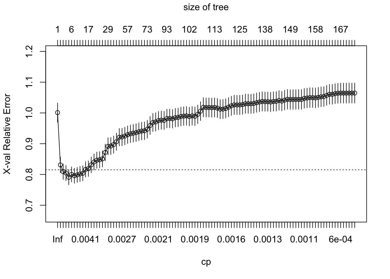

The following code retrieves the optimal parameter and prunes the tree.

# Retrieves the optimal parameter
cp.idx <- which.min(tree$cptable[,"xerror"])
cp.best <- tree$cptable[cp.idx,"CP"]  

# Prune the tree
pruned.tree <- prune(tree, cp=cp.best)

Plotting the pruned tree. See also the package rpart.plot for more advanced plotting capabilities.

plot(pruned.tree, uniform=TRUE, margin = .05)
text(pruned.tree, cex=.7)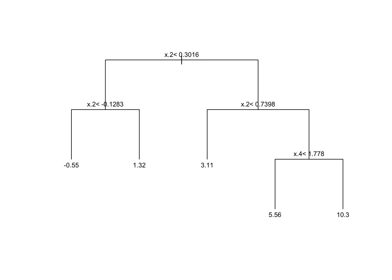

Finally, here’s how to extract predictions and mse estimates from the pruned tree.

# Retrieve predictions from pruned tree
y.hat <- predict(pruned.tree)

# Compute mse for pruned tree (using cross-validated predictions)
mse.tree <- mean((xpred.rpart(tree)[,cp.idx] - data$y)^2)
print(paste("Tree MSE estimate (cross-validated):", mse.tree))

## [1] "Tree MSE estimate (cross-validated): 21.4581149379238"

It’s often said that trees are “interpretable.” To some extent, that’s true – we can look at the tree and clearly visualize the mapping from inputs to prediction. This can be important in settings in which conveying how one got to a prediction is important. For example, if a decision tree were to be used for credit scoring, it would be easy to explain to a client how their credit was scored.

However, beyond that we should not trying to interpreting the estimated decision tree, for several reasons. First, even though a tree may have used a particular variable for a split, that does not mean that it’s indeed an important variable: if two covariates are highly correlated, the tree may split on one variable but not the other, and there’s no guarantee which variables are actually relevant in the underlying data-generating process. Moreover, many tree algorithms have other issues such as favoring continuous variables over binary ones, because continuous variables more opportunities to find a split that (possibly spuriously) seems good.

2.2.2 Generalized linear models

The next class of models extends common methods such as linear and logistic regression by adding a penalty to the magnitude of the coefficients. Lasso penalizes the absolute value of slope coefficients. For regression problems, it becomes \[\begin{equation} \tag{2.3} \hat{b}_{Lasso} = \arg\min_b \sum_{i=1}^m \left(Y_i - b_0 - \sum_{j=1}^{p} X_{ij} b_j \right)^2 + \lambda \sum_{j=1}^{p} |b_j|. \end{equation}\]

Similarly, in a regression problem Ridge penalizes the sum of squares of the slope coefficients, \[\begin{equation} \tag{2.4} \hat{b}_{Ridge} = \arg\min_b \sum_{i=1}^m \left(Y_i - b_0 - \sum_{j=1}^{p} X_{ij} b_j \right)^2 + \lambda \sum_{j=1}^{p} b_j^2. \end{equation}\]

In addition, there are exist the Elastic Net penalization which consists of a convex combination between the other two. In all cases, the scalar parameter \(\lambda\) controls the complexity of the model. For \(\lambda = 0\), the problem reduces to the “usual” linear regression. As \(\lambda\) increases, we favor simpler models. As we’ll see below, the optimal parameter \(\lambda\) is selected via cross-validation.

An important feature of Lasso-type penalization is that it promotes sparsity – that is, it forces many coefficients to be exactly zero. This is different from Ridge-type penalization, which forces coefficients to be small.

Another interesting property of these models is that, even though they are called “linear” models, this should actually be understood as linear in transformations of the covariates. For example, we could use polynomials or splines (continuous piecewise polynomials) of the covariates and allow for much more flexible models.

In fact, because of the penalization term, problems (2.3) and (2.4) remain well-defined and have a unique solution even in high-dimensional problem in which the number of coefficients \(p\) is larger than the sample size \(n\) – that is, our data “fat” with more columns than rows. These situations can arise either naturally (e.g. genomics problems in which we have hundreds of thousands of gene expression information for a few individuals) or because we are including many transformations of a smaller set of covariates.

Finally, although here we are focusing on regression problems, other generalized linear model such as logistic regression can also be similarly modified by adding a Lasso, Ridge or Elastic Net-type penalty to similar consequences.

In our example we will use the glmnet package; see this excellent tutorial for more information about the package, including how to use glmnet for other types of outcomes (binomial, categorical, multi-valued). The function cv.glmnet automatically performs k-fold cross-validation. Also, to emphasize the point about linearity “in transformations” of the covariates, we will use splines of our independent variables (i.e., we will use piecewise continuous polynomials of the original covariates). This is done using the function bs; see this primer for more information.

# Create a matrix of features based on spline transformations of covariates
fmla <- formula(paste(" ~ 0 + ", paste0("bs(", covariates, ", df=5)", collapse=" + ")))
XX <- model.matrix(fmla, data)
Y <- data[, outcome]

# Fit a lasso model
lasso <- cv.glmnet(
  x=XX, y=Y, 
  family="gaussian", # use 'binomial' for logistic regression
  alpha=1. # use alpha=0 for ridge, or alpha in (0, 1) for elastic net
)

Here’s a plot of the magnitude of each coefficient as we vary the \(\lambda\) paramter. Note how for higher values of \(\lambda\) many coefficients become exactly zero.

plot(lasso$glmnet.fit, xvar="lambda")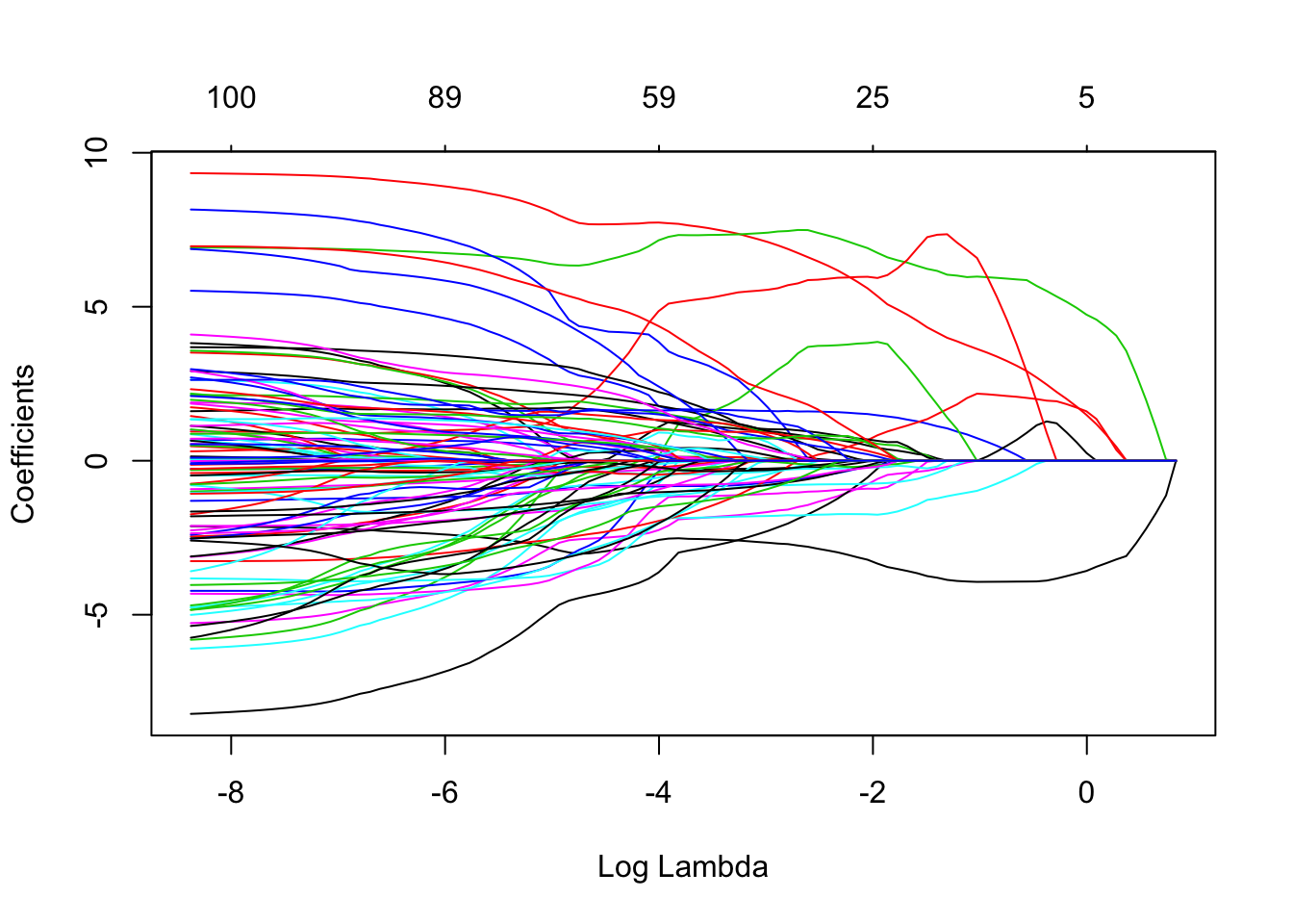

The next figure plots the average estimated MSE for each lambda. The red dots are the averages across all folds, and the error bars are based on the variability of mse estimates across folds. The vertical dashed lines shows the (log) lambda with smallest estimated MSE (left) and the one whose mse is at most one standard error from the first (right).

plot(lasso)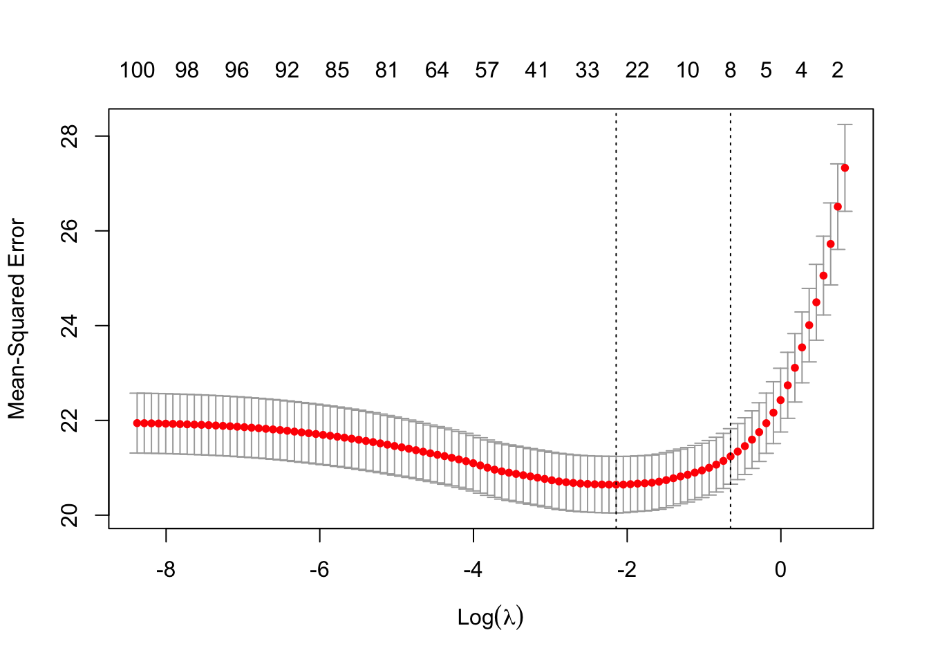

Here are the first ten estimated coefficients. Note how many of them are zero.

# Estimated coefficients at the lambda value that minimized cross-validated MSE
coef(lasso, s = "lambda.min")[1:10,]  # showing only first ten coefficients

##      (Intercept) bs(x.1, df = 5)1 bs(x.1, df = 5)2 bs(x.1, df = 5)3 
##        2.3644243       -0.0784574        0.0000000        0.0000000 
## bs(x.1, df = 5)4 bs(x.1, df = 5)5 bs(x.2, df = 5)1 bs(x.2, df = 5)2 
##        1.5354613        0.0000000        0.0000000       -3.1365320 
## bs(x.2, df = 5)3 bs(x.2, df = 5)4 
##        5.8057386        7.0105914

Finally, the predictions and estimated MSE for the selected model are retrieved as follows.

# Retrieve predictions at best lambda regularization parameter
y.hat <- predict(lasso, newx=XX, s="lambda.min", type="response")

# Get k-fold cross validation 
mse.glmnet <-  lasso$cvm[lasso$lambda == lasso$lambda.min]
print(paste("glmnet MSE estimate (k-fold cross-validation):", mse.glmnet))

## [1] "glmnet MSE estimate (k-fold cross-validation): 20.6430792177004"

We recommend avoid interpreting the Lasso coefficients. Similar to what we saw above with trees, when multiple covariates are highly correlated the model may decide to spuriously “drop” several of them by forcing its coefficient to be zero). As discussed in Mullainathan and Spiess (JEP, 2017), there may be many choices of coefficients with similar predictive power, so the set of nonzero coefficients we end up with can be quite unstable (for illustration, you may want to change the seed at the beginning of this chapter, rerun the code and see this phenomenon by yourself). This means that we should not use the Lasso model for computing partial effects either. In addition, dropping covariates can lead to a form of ommitted variable bias. To a great extent, these issues remain even if we use Ridge or Elastic Net, so we caution against interpreting those models as well. That said, although we won’t be covering it in this tutorial, there has been a lot of research on inference in high-dimensional models; see e.g., Belloni, Chernozhukov and Hansen (JEP, 2014 and the accompanying R package hdm.

2.2.3 Forests

Forests are a type of ensemble estimators: they aggregate information about many decision trees to compute a new estimate that typically has much smaller variance.

At a high level, the process of fitting a (regression) forest consists of fitting many decision trees, each on a different subsample of the data. The forest prediction for a particular point \(x\) is the average of all tree predictions for that point [1].

One interesting aspect of forests and many other ensemble methods is that cross-validation can be built into the algorithm itself. Since each tree only uses a subset of the data, the remaining subset is effectively a test set for that tree. We call these observations out-of-bag (there were not in the “bag” of training observations). They can be used to evaluate the performance of that tree, and the average of out-of-bag evaluations is evidence of the performance of the forest itself.

For the example below, we’ll use the regression_forest function of the R package grf. This particular implementation in grf has other interesting. For example, trees are build using a certain sample-splitting scheme that ensures that predictions are approximately unbiased and normally distributed for large samples, which in turn allows us to compute valid confidence intervals around those predictions. We’ll have more to say about the importance of these features when we talk about causal estimates in future chapters. See also the grf website for more information.

X <- data[,covariates]
Y <- data[,outcome]

# Fitting the forest
forest <- regression_forest(X=X, Y=Y) 

# There usually isn't a lot of benefit in tuning forest parameters, but the next code does so automatically (expect longer training times)
# forest <- regression_forest(X=X, Y=Y, tune.parameters="all")

# Retrieving forest predictions
y.hat <- predict(forest)$predictions

# Evaluation (out-of-bag mse)
mse.oob <- mean(predict(forest)$debiased.error)
print(paste("Forest MSE (out-of-bag):", mse.oob))

## [1] "Forest MSE (out-of-bag): 20.6845675952809"

The funcion variable_importance computes a simple weighted sum of how many times each feature was split on at each depth across the trees.

var.imp <- variable_importance(forest)
names(var.imp) <- covariates
sort(var.imp, decreasing = TRUE)[1:10]

##        x.2        x.3        x.4        x.1        x.5       x.11       x.13 
## 0.72693496 0.07191355 0.05120252 0.04718775 0.01820078 0.00774203 0.00734184 
##        x.6        x.7        x.8 
## 0.00657309 0.00640645 0.00635314

All the caveats about interpretation that we mentioned above apply in a similar to forest output.

2.3 Further reading

James, G., Witten, D., Hastie, T., & Tibshirani, R. (2013). An introduction to statistical learning (Vol. 112, p. 18). New York: springer. Available for free at the authors’ website.

2.4 Notes

[1] There are two ways of understanding what happens at prediction time. One is that the final prediction is the average of the predictions from each tree for a particular point \(x\). The other is that tree partitions induce a notion of “neighborhood”: the prediction at a point \(x\) is the average of all outcomes \(Y_i\) in the data set, weighted by how often the covariates observation \(i\) shared a terminal node with point \(x\).