Chapter 30 Statistical Tests

What You’ll Learn:

t-tests (one-sample, two-sample, paired)
Common statistical test errors
Assumptions and violations
Interpreting results
Effect sizes

Key Errors Covered: 22+ statistical errors

Difficulty: ⭐⭐ Intermediate to ⭐⭐⭐ Advanced

30.1 Introduction

R excels at statistical testing, but errors are common:

# Simple t-test
t.test(mtcars$mpg[mtcars$am == 0], 
       mtcars$mpg[mtcars$am == 1])
#> 
#>  Welch Two Sample t-test
#> 
#> data:  mtcars$mpg[mtcars$am == 0] and mtcars$mpg[mtcars$am == 1]
#> t = -3.7671, df = 18.332, p-value = 0.001374
#> alternative hypothesis: true difference in means is not equal to 0
#> 95 percent confidence interval:
#>  -11.280194  -3.209684
#> sample estimates:
#> mean of x mean of y 
#>  17.14737  24.39231

Let’s master statistical testing errors!

30.2 t-tests

💡 Key Insight: Types of t-tests

# One-sample t-test (compare to population mean)
t.test(mtcars$mpg, mu = 20)
#> 
#>  One Sample t-test
#> 
#> data:  mtcars$mpg
#> t = 0.08506, df = 31, p-value = 0.9328
#> alternative hypothesis: true mean is not equal to 20
#> 95 percent confidence interval:
#>  17.91768 22.26357
#> sample estimates:
#> mean of x 
#>  20.09062

# Two-sample t-test (independent groups)
t.test(mpg ~ am, data = mtcars)
#> 
#>  Welch Two Sample t-test
#> 
#> data:  mpg by am
#> t = -3.7671, df = 18.332, p-value = 0.001374
#> alternative hypothesis: true difference in means between group 0 and group 1 is not equal to 0
#> 95 percent confidence interval:
#>  -11.280194  -3.209684
#> sample estimates:
#> mean in group 0 mean in group 1 
#>        17.14737        24.39231

# Paired t-test (same subjects, two conditions)
before <- c(120, 135, 140, 125, 130)
after <- c(115, 130, 135, 120, 128)
t.test(before, after, paired = TRUE)
#> 
#>  Paired t-test
#> 
#> data:  before and after
#> t = 7.3333, df = 4, p-value = 0.001841
#> alternative hypothesis: true mean difference is not equal to 0
#> 95 percent confidence interval:
#>  2.734133 6.065867
#> sample estimates:
#> mean difference 
#>             4.4

# One-sided test
t.test(mpg ~ am, data = mtcars, alternative = "greater")
#> 
#>  Welch Two Sample t-test
#> 
#> data:  mpg by am
#> t = -3.7671, df = 18.332, p-value = 0.9993
#> alternative hypothesis: true difference in means between group 0 and group 1 is greater than 0
#> 95 percent confidence interval:
#>  -10.57662       Inf
#> sample estimates:
#> mean in group 0 mean in group 1 
#>        17.14737        24.39231

# Unequal variances (Welch's t-test, default)
t.test(mpg ~ am, data = mtcars, var.equal = FALSE)
#> 
#>  Welch Two Sample t-test
#> 
#> data:  mpg by am
#> t = -3.7671, df = 18.332, p-value = 0.001374
#> alternative hypothesis: true difference in means between group 0 and group 1 is not equal to 0
#> 95 percent confidence interval:
#>  -11.280194  -3.209684
#> sample estimates:
#> mean in group 0 mean in group 1 
#>        17.14737        24.39231

# Equal variances (Student's t-test)
t.test(mpg ~ am, data = mtcars, var.equal = TRUE)
#> 
#>  Two Sample t-test
#> 
#> data:  mpg by am
#> t = -4.1061, df = 30, p-value = 0.000285
#> alternative hypothesis: true difference in means between group 0 and group 1 is not equal to 0
#> 95 percent confidence interval:
#>  -10.84837  -3.64151
#> sample estimates:
#> mean in group 0 mean in group 1 
#>        17.14737        24.39231

30.3 Error #1: `not enough 'x' observations`

⭐ BEGINNER 📊 DATA

30.3.1 The Error

# Only one observation
t.test(c(5))
#> Error in t.test.default(c(5)): not enough 'x' observations

🔴 ERROR

Error in t.test.default(c(5)) : not enough 'x' observations

30.3.2 What It Means

Need at least 2 observations for t-test.

30.3.3 Common Causes

# Empty vector after filtering
data <- mtcars$mpg[mtcars$cyl == 99]  # No cars with 99 cylinders
t.test(data)
#> Error in t.test.default(data): not enough 'x' observations

# Single group
t.test(mtcars$mpg[mtcars$am == 0], mtcars$mpg[mtcars$am == 99])
#> Error in t.test.default(mtcars$mpg[mtcars$am == 0], mtcars$mpg[mtcars$am == : not enough 'y' observations

30.3.4 Solutions

✅ SOLUTION 1: Check Data First

# Check sample sizes
automatic <- mtcars$mpg[mtcars$am == 0]
manual <- mtcars$mpg[mtcars$am == 1]

cat("Automatic:", length(automatic), "observations\n")
#> Automatic: 19 observations
cat("Manual:", length(manual), "observations\n")
#> Manual: 13 observations

if (length(automatic) >= 2 && length(manual) >= 2) {
  t.test(automatic, manual)
} else {
  warning("Insufficient data for t-test")
}
#> 
#>  Welch Two Sample t-test
#> 
#> data:  automatic and manual
#> t = -3.7671, df = 18.332, p-value = 0.001374
#> alternative hypothesis: true difference in means is not equal to 0
#> 95 percent confidence interval:
#>  -11.280194  -3.209684
#> sample estimates:
#> mean of x mean of y 
#>  17.14737  24.39231

✅ SOLUTION 2: Safe t-test Function

safe_t_test <- function(x, y = NULL, ...) {
  if (is.null(y)) {
    if (length(x) < 2) {
      stop("x must have at least 2 observations")
    }
  } else {
    if (length(x) < 2) {
      stop("x must have at least 2 observations")
    }
    if (length(y) < 2) {
      stop("y must have at least 2 observations")
    }
  }
  
  t.test(x, y, ...)
}

# Test
safe_t_test(mtcars$mpg[mtcars$am == 0], 
            mtcars$mpg[mtcars$am == 1])
#> 
#>  Welch Two Sample t-test
#> 
#> data:  x and y
#> t = -3.7671, df = 18.332, p-value = 0.001374
#> alternative hypothesis: true difference in means is not equal to 0
#> 95 percent confidence interval:
#>  -11.280194  -3.209684
#> sample estimates:
#> mean of x mean of y 
#>  17.14737  24.39231

30.4 Error #2: `data are essentially constant`

⭐⭐ INTERMEDIATE 📊 DATA

30.4.1 The Error

# All values the same
t.test(c(5, 5, 5, 5, 5))
#> Error in t.test.default(c(5, 5, 5, 5, 5)): data are essentially constant

🔴 ERROR

Error in t.test.default(c(5, 5, 5, 5, 5)) : 
  data are essentially constant

30.4.2 What It Means

No variation in data - standard deviation is zero or near-zero.

30.4.3 Common Causes

# Rounded data with no variation
t.test(c(10, 10, 10, 10, 10))
#> Error in t.test.default(c(10, 10, 10, 10, 10)): data are essentially constant

# Binary data coded as 0/1 with all same
t.test(c(1, 1, 1, 1))
#> Error in t.test.default(c(1, 1, 1, 1)): data are essentially constant

30.4.4 Solutions

✅ SOLUTION 1: Check for Variation

check_variation <- function(x) {
  if (sd(x) == 0 || length(unique(x)) == 1) {
    warning("No variation in data - t-test not appropriate")
    return(FALSE)
  }
  TRUE
}

# Check before test
data <- c(10, 10, 10, 10)
if (check_variation(data)) {
  t.test(data)
} else {
  cat("Data has no variation\n")
}
#> Warning in check_variation(data): No variation in data - t-test not appropriate
#> Data has no variation

✅ SOLUTION 2: Use Appropriate Test

# For proportions, use prop.test
successes <- c(1, 1, 1, 1)  # All successes
prop.test(sum(successes), length(successes))
#> Warning in prop.test(sum(successes), length(successes)): Chi-squared
#> approximation may be incorrect
#> 
#>  1-sample proportions test with continuity correction
#> 
#> data:  sum(successes) out of length(successes), null probability 0.5
#> X-squared = 2.25, df = 1, p-value = 0.1336
#> alternative hypothesis: true p is not equal to 0.5
#> 95 percent confidence interval:
#>  0.395773 1.000000
#> sample estimates:
#> p 
#> 1

# Or check if variation exists
data <- mtcars$mpg
if (sd(data) > 0) {
  t.test(data, mu = 20)
} else {
  cat("Data is constant, mean =", mean(data), "\n")
}
#> 
#>  One Sample t-test
#> 
#> data:  data
#> t = 0.08506, df = 31, p-value = 0.9328
#> alternative hypothesis: true mean is not equal to 20
#> 95 percent confidence interval:
#>  17.91768 22.26357
#> sample estimates:
#> mean of x 
#>  20.09062

30.5 Formula Interface

💡 Key Insight: Formula vs Vector Interface

# Vector interface
group1 <- mtcars$mpg[mtcars$am == 0]
group2 <- mtcars$mpg[mtcars$am == 1]
t.test(group1, group2)
#> 
#>  Welch Two Sample t-test
#> 
#> data:  group1 and group2
#> t = -3.7671, df = 18.332, p-value = 0.001374
#> alternative hypothesis: true difference in means is not equal to 0
#> 95 percent confidence interval:
#>  -11.280194  -3.209684
#> sample estimates:
#> mean of x mean of y 
#>  17.14737  24.39231

# Formula interface (preferred)
t.test(mpg ~ am, data = mtcars)
#> 
#>  Welch Two Sample t-test
#> 
#> data:  mpg by am
#> t = -3.7671, df = 18.332, p-value = 0.001374
#> alternative hypothesis: true difference in means between group 0 and group 1 is not equal to 0
#> 95 percent confidence interval:
#>  -11.280194  -3.209684
#> sample estimates:
#> mean in group 0 mean in group 1 
#>        17.14737        24.39231

# Formula with subset
t.test(mpg ~ am, data = mtcars, subset = cyl == 4)
#> 
#>  Welch Two Sample t-test
#> 
#> data:  mpg by am
#> t = -2.8855, df = 8.9993, p-value = 0.01802
#> alternative hypothesis: true difference in means between group 0 and group 1 is not equal to 0
#> 95 percent confidence interval:
#>  -9.232108 -1.117892
#> sample estimates:
#> mean in group 0 mean in group 1 
#>          22.900          28.075

# Advantages of formula:
# - Cleaner code
# - Automatic labeling
# - Works with model functions
# - Subset argument

30.6 Error #3: `grouping factor must have 2 levels`

⭐ BEGINNER 📊 DATA

30.6.1 The Error

# Three levels in grouping variable
t.test(mpg ~ cyl, data = mtcars)
#> Error in t.test.formula(mpg ~ cyl, data = mtcars): grouping factor must have exactly 2 levels

🔴 ERROR

Error in t.test.formula(mpg ~ cyl, data = mtcars) : 
  grouping factor must have exactly 2 levels

30.6.2 What It Means

t-test compares exactly 2 groups. Variable has more than 2 levels.

30.6.3 Solutions

✅ SOLUTION 1: Filter to 2 Groups

# Compare only 4 vs 6 cylinders
mtcars_subset <- mtcars[mtcars$cyl %in% c(4, 6), ]
t.test(mpg ~ cyl, data = mtcars_subset)
#> 
#>  Welch Two Sample t-test
#> 
#> data:  mpg by cyl
#> t = 4.7191, df = 12.956, p-value = 0.0004048
#> alternative hypothesis: true difference in means between group 4 and group 6 is not equal to 0
#> 95 percent confidence interval:
#>   3.751376 10.090182
#> sample estimates:
#> mean in group 4 mean in group 6 
#>        26.66364        19.74286

# Or use subset argument
t.test(mpg ~ cyl, data = mtcars, subset = cyl %in% c(4, 6))
#> 
#>  Welch Two Sample t-test
#> 
#> data:  mpg by cyl
#> t = 4.7191, df = 12.956, p-value = 0.0004048
#> alternative hypothesis: true difference in means between group 4 and group 6 is not equal to 0
#> 95 percent confidence interval:
#>   3.751376 10.090182
#> sample estimates:
#> mean in group 4 mean in group 6 
#>        26.66364        19.74286

✅ SOLUTION 2: Use ANOVA for >2 Groups

# For 3+ groups, use ANOVA
anova_result <- aov(mpg ~ factor(cyl), data = mtcars)
summary(anova_result)
#>             Df Sum Sq Mean Sq F value   Pr(>F)    
#> factor(cyl)  2  824.8   412.4    39.7 4.98e-09 ***
#> Residuals   29  301.3    10.4                     
#> ---
#> Signif. codes:  0 '***' 0.001 '**' 0.01 '*' 0.05 '.' 0.1 ' ' 1

# Post-hoc tests
TukeyHSD(anova_result)
#>   Tukey multiple comparisons of means
#>     95% family-wise confidence level
#> 
#> Fit: aov(formula = mpg ~ factor(cyl), data = mtcars)
#> 
#> $`factor(cyl)`
#>           diff        lwr        upr     p adj
#> 6-4  -6.920779 -10.769350 -3.0722086 0.0003424
#> 8-4 -11.563636 -14.770779 -8.3564942 0.0000000
#> 8-6  -4.642857  -8.327583 -0.9581313 0.0112287

✅ SOLUTION 3: Multiple Comparisons

# Compare all pairs
library(dplyr)

# Get unique cylinder values
cyl_levels <- unique(mtcars$cyl)
comparisons <- combn(cyl_levels, 2)

# Perform all pairwise tests
results <- apply(comparisons, 2, function(pair) {
  subset_data <- mtcars[mtcars$cyl %in% pair, ]
  test <- t.test(mpg ~ cyl, data = subset_data)
  
  data.frame(
    comparison = paste(pair[1], "vs", pair[2]),
    p_value = test$p.value,
    statistic = test$statistic
  )
})

do.call(rbind, results)
#>    comparison      p_value statistic
#> t      6 vs 4 4.048495e-04  4.719059
#> t1     6 vs 8 4.540355e-05  5.291135
#> t2     4 vs 8 1.641348e-06  7.596664

30.7 Assumptions

💡 Key Insight: t-test Assumptions

# Assumptions:
# 1. Independence
# 2. Normality (esp. for small samples)
# 3. Equal variances (for Student's t-test)

# Check normality
shapiro.test(mtcars$mpg)
#> 
#>  Shapiro-Wilk normality test
#> 
#> data:  mtcars$mpg
#> W = 0.94756, p-value = 0.1229

# Visual check
qqnorm(mtcars$mpg)
qqline(mtcars$mpg)

# Check equal variances
var.test(mpg ~ am, data = mtcars)
#> 
#>  F test to compare two variances
#> 
#> data:  mpg by am
#> F = 0.38656, num df = 18, denom df = 12, p-value = 0.06691
#> alternative hypothesis: true ratio of variances is not equal to 1
#> 95 percent confidence interval:
#>  0.1243721 1.0703429
#> sample estimates:
#> ratio of variances 
#>          0.3865615

# If assumptions violated:
# - Use Welch's t-test (var.equal = FALSE, default)
# - Use Mann-Whitney U test (non-parametric)
wilcox.test(mpg ~ am, data = mtcars)
#> Warning in wilcox.test.default(x = DATA[[1L]], y = DATA[[2L]], ...): cannot
#> compute exact p-value with ties
#> 
#>  Wilcoxon rank sum test with continuity correction
#> 
#> data:  mpg by am
#> W = 42, p-value = 0.001871
#> alternative hypothesis: true location shift is not equal to 0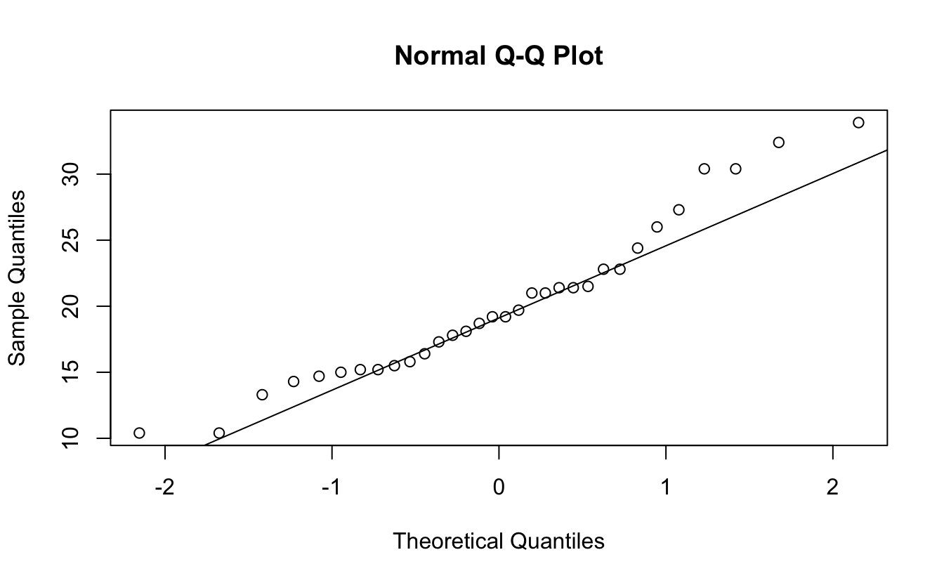

30.8 Interpreting Results

💡 Key Insight: Understanding Output

result <- t.test(mpg ~ am, data = mtcars)
result
#> 
#>  Welch Two Sample t-test
#> 
#> data:  mpg by am
#> t = -3.7671, df = 18.332, p-value = 0.001374
#> alternative hypothesis: true difference in means between group 0 and group 1 is not equal to 0
#> 95 percent confidence interval:
#>  -11.280194  -3.209684
#> sample estimates:
#> mean in group 0 mean in group 1 
#>        17.14737        24.39231

# Extract components
result$statistic    # t-statistic
#>         t 
#> -3.767123
result$parameter    # degrees of freedom
#>       df 
#> 18.33225
result$p.value      # p-value
#> [1] 0.001373638
result$conf.int     # confidence interval
#> [1] -11.280194  -3.209684
#> attr(,"conf.level")
#> [1] 0.95
result$estimate     # group means
#> mean in group 0 mean in group 1 
#>        17.14737        24.39231

# Interpretation
cat("t-statistic:", round(result$statistic, 3), "\n")
#> t-statistic: -3.767
cat("p-value:", round(result$p.value, 4), "\n")
#> p-value: 0.0014
cat("95% CI:", round(result$conf.int, 2), "\n")
#> 95% CI: -11.28 -3.21
cat("Mean difference:", round(diff(result$estimate), 2), "\n")
#> Mean difference: 7.24

if (result$p.value < 0.05) {
  cat("\nSignificant difference between groups (p < 0.05)\n")
} else {
  cat("\nNo significant difference between groups (p >= 0.05)\n")
}
#> 
#> Significant difference between groups (p < 0.05)

30.9 Effect Size

🎯 Best Practice: Report Effect Sizes

# Cohen's d for effect size
cohens_d <- function(x, y) {
  n1 <- length(x)
  n2 <- length(y)
  
  # Pooled standard deviation
  s_pooled <- sqrt(((n1 - 1) * var(x) + (n2 - 1) * var(y)) / (n1 + n2 - 2))
  
  # Cohen's d
  d <- (mean(x) - mean(y)) / s_pooled
  
  # Interpretation
  interpretation <- if (abs(d) < 0.2) "negligible"
    else if (abs(d) < 0.5) "small"
    else if (abs(d) < 0.8) "medium"
    else "large"
  
  list(
    d = d,
    interpretation = interpretation
  )
}

# Calculate effect size
auto <- mtcars$mpg[mtcars$am == 0]
manual <- mtcars$mpg[mtcars$am == 1]

effect <- cohens_d(auto, manual)
cat("Cohen's d:", round(effect$d, 2), "\n")
#> Cohen's d: -1.48
cat("Effect size:", effect$interpretation, "\n")
#> Effect size: large

30.10 Paired t-tests

💡 Key Insight: Paired vs Independent

# Paired: same subjects, two conditions
before <- c(120, 135, 140, 125, 130, 145, 150)
after <- c(115, 130, 135, 120, 128, 140, 145)

# Paired t-test
t.test(before, after, paired = TRUE)
#> 
#>  Paired t-test
#> 
#> data:  before and after
#> t = 10.667, df = 6, p-value = 4.004e-05
#> alternative hypothesis: true mean difference is not equal to 0
#> 95 percent confidence interval:
#>  3.522752 5.620105
#> sample estimates:
#> mean difference 
#>        4.571429

# Calculate differences
differences <- before - after
cat("Mean difference:", mean(differences), "\n")
#> Mean difference: 4.571429
cat("SD of differences:", sd(differences), "\n")
#> SD of differences: 1.133893

# One-sample test on differences (equivalent)
t.test(differences, mu = 0)
#> 
#>  One Sample t-test
#> 
#> data:  differences
#> t = 10.667, df = 6, p-value = 4.004e-05
#> alternative hypothesis: true mean is not equal to 0
#> 95 percent confidence interval:
#>  3.522752 5.620105
#> sample estimates:
#> mean of x 
#>  4.571429

# Independent would be WRONG here
t.test(before, after, paired = FALSE)  # Ignores pairing
#> 
#>  Welch Two Sample t-test
#> 
#> data:  before and after
#> t = 0.79817, df = 11.997, p-value = 0.4403
#> alternative hypothesis: true difference in means is not equal to 0
#> 95 percent confidence interval:
#>  -7.907792 17.050649
#> sample estimates:
#> mean of x mean of y 
#>  135.0000  130.4286

30.11 Error #4: `'x' and 'y' must have the same length`

⭐ BEGINNER 📊 DATA

30.11.1 The Error

before <- c(120, 135, 140, 125)
after <- c(115, 130, 135)  # Only 3 values

t.test(before, after, paired = TRUE)
#> Error in complete.cases(x, y): not all arguments have the same length

🔴 ERROR

Error in t.test.default(before, after, paired = TRUE) : 
  'x' and 'y' must have the same length

30.11.2 What It Means

Paired t-test requires same number of observations in each group.

30.11.3 Solutions

✅ SOLUTION 1: Check Lengths

before <- c(120, 135, 140, 125, 130)
after <- c(115, 130, 135, 120, 128)

if (length(before) != length(after)) {
  stop("before and after must have same length for paired test")
}

t.test(before, after, paired = TRUE)
#> 
#>  Paired t-test
#> 
#> data:  before and after
#> t = 7.3333, df = 4, p-value = 0.001841
#> alternative hypothesis: true mean difference is not equal to 0
#> 95 percent confidence interval:
#>  2.734133 6.065867
#> sample estimates:
#> mean difference 
#>             4.4

✅ SOLUTION 2: Handle Missing Data

# Data with NAs
before <- c(120, 135, NA, 125, 130)
after <- c(115, 130, 135, 120, NA)

# Remove pairs with any NA
complete_cases <- complete.cases(before, after)
before_clean <- before[complete_cases]
after_clean <- after[complete_cases]

cat("Complete pairs:", sum(complete_cases), "\n")
#> Complete pairs: 3

t.test(before_clean, after_clean, paired = TRUE)
#> Error in t.test.default(before_clean, after_clean, paired = TRUE): data are essentially constant

✅ SOLUTION 3: Use Data Frame Approach

library(dplyr)
library(tidyr)

# Store in data frame
data <- data.frame(
  id = 1:5,
  before = c(120, 135, NA, 125, 130),
  after = c(115, 130, 135, 120, NA)
)

# Remove incomplete cases
data_complete <- data %>%
  filter(!is.na(before) & !is.na(after))

cat("Complete cases:", nrow(data_complete), "\n")
#> Complete cases: 3

with(data_complete, t.test(before, after, paired = TRUE))
#> Error in t.test.default(before, after, paired = TRUE): data are essentially constant

30.12 Power and Sample Size

🎯 Best Practice: Power Analysis

# Calculate required sample size
power.t.test(
  delta = 5,        # Expected difference
  sd = 10,          # Standard deviation
  sig.level = 0.05, # Alpha
  power = 0.80      # Desired power
)
#> 
#>      Two-sample t test power calculation 
#> 
#>               n = 63.76576
#>           delta = 5
#>              sd = 10
#>       sig.level = 0.05
#>           power = 0.8
#>     alternative = two.sided
#> 
#> NOTE: n is number in *each* group

# Calculate power for given sample size
power.t.test(
  n = 20,
  delta = 5,
  sd = 10,
  sig.level = 0.05
)
#> 
#>      Two-sample t test power calculation 
#> 
#>               n = 20
#>           delta = 5
#>              sd = 10
#>       sig.level = 0.05
#>           power = 0.3377084
#>     alternative = two.sided
#> 
#> NOTE: n is number in *each* group

# For existing study
auto <- mtcars$mpg[mtcars$am == 0]
manual <- mtcars$mpg[mtcars$am == 1]

power.t.test(
  n = length(auto),
  delta = abs(mean(auto) - mean(manual)),
  sd = sd(c(auto, manual)),
  sig.level = 0.05
)
#> 
#>      Two-sample t test power calculation 
#> 
#>               n = 19
#>           delta = 7.244939
#>              sd = 6.026948
#>       sig.level = 0.05
#>           power = 0.9499733
#>     alternative = two.sided
#> 
#> NOTE: n is number in *each* group

30.13 Summary

Key Takeaways:

Check sample sizes - Need at least 2 observations per group
Check variation - Data can’t be constant
Exactly 2 groups - Use ANOVA for 3+
Paired = same length - Remove incomplete pairs
Check assumptions - Normality, equal variances
Report effect sizes - Not just p-values
Formula interface preferred - Cleaner code

Quick Reference:

Error	Cause	Fix
not enough observations	n < 2	Check sample sizes
data are constant	sd = 0	Check for variation
must have 2 levels	3+ groups	Filter or use ANOVA
must have same length	Paired mismatch	Remove incomplete pairs

t-test Variations:

# One-sample
t.test(x, mu = 0)

# Two-sample (independent)
t.test(x, y)
t.test(y ~ x, data = df)

# Paired
t.test(x, y, paired = TRUE)

# One-sided
t.test(x, y, alternative = "greater")
t.test(x, y, alternative = "less")

# Equal variances
t.test(x, y, var.equal = TRUE)

# With subset
t.test(y ~ x, data = df, subset = condition)

Best Practices:

# ✅ Good
Check sample sizes first
Check assumptions (normality, equal variance)
Use formula interface: t.test(y ~ x, data = df)
Report effect sizes (Cohen's d)
Use Welch's t-test (default) for unequal variances
Check for paired vs independent design

# ❌ Avoid
Assuming data meets assumptions
Using t-test for 3+ groups
Ignoring pairing in data
Only reporting p-values
Using with constant data
Not checking sample sizes

30.14 Exercises

📝 Exercise 1: Basic t-test

Using mtcars: 1. Test if mean mpg differs by transmission (am) 2. Check assumptions 3. Calculate effect size 4. Interpret results

📝 Exercise 2: Paired t-test

Create before/after data and: 1. Perform paired t-test 2. Check if order matters 3. Calculate mean difference 4. Visualize differences

📝 Exercise 3: Safe t-test Function

Write safe_t_test() that: 1. Checks sample sizes 2. Checks for variation 3. Verifies assumptions 4. Performs test 5. Returns formatted results

📝 Exercise 4: Multiple Comparisons

Using iris dataset: 1. Compare petal length across species 2. Perform all pairwise t-tests 3. Adjust for multiple testing 4. Report results in table

30.15 Exercise Answers

Click to see answers

Exercise 1:

# 1. Test mean mpg by transmission
result <- t.test(mpg ~ am, data = mtcars)
result
#> 
#>  Welch Two Sample t-test
#> 
#> data:  mpg by am
#> t = -3.7671, df = 18.332, p-value = 0.001374
#> alternative hypothesis: true difference in means between group 0 and group 1 is not equal to 0
#> 95 percent confidence interval:
#>  -11.280194  -3.209684
#> sample estimates:
#> mean in group 0 mean in group 1 
#>        17.14737        24.39231

# 2. Check assumptions
# Normality
shapiro.test(mtcars$mpg[mtcars$am == 0])
#> 
#>  Shapiro-Wilk normality test
#> 
#> data:  mtcars$mpg[mtcars$am == 0]
#> W = 0.97677, p-value = 0.8987
shapiro.test(mtcars$mpg[mtcars$am == 1])
#> 
#>  Shapiro-Wilk normality test
#> 
#> data:  mtcars$mpg[mtcars$am == 1]
#> W = 0.9458, p-value = 0.5363

# Equal variances
var.test(mpg ~ am, data = mtcars)
#> 
#>  F test to compare two variances
#> 
#> data:  mpg by am
#> F = 0.38656, num df = 18, denom df = 12, p-value = 0.06691
#> alternative hypothesis: true ratio of variances is not equal to 1
#> 95 percent confidence interval:
#>  0.1243721 1.0703429
#> sample estimates:
#> ratio of variances 
#>          0.3865615

# 3. Effect size
auto <- mtcars$mpg[mtcars$am == 0]
manual <- mtcars$mpg[mtcars$am == 1]

cohens_d <- function(x, y) {
  n1 <- length(x)
  n2 <- length(y)
  s_pooled <- sqrt(((n1 - 1) * var(x) + (n2 - 1) * var(y)) / (n1 + n2 - 2))
  (mean(x) - mean(y)) / s_pooled
}

d <- cohens_d(auto, manual)

# 4. Interpret
cat("\n=== Results ===\n")
#> 
#> === Results ===
cat("t-statistic:", round(result$statistic, 3), "\n")
#> t-statistic: -3.767
cat("p-value:", format.pval(result$p.value, digits = 3), "\n")
#> p-value: 0.00137
cat("Mean difference:", round(diff(result$estimate), 2), "mpg\n")
#> Mean difference: 7.24 mpg
cat("95% CI:", round(result$conf.int, 2), "\n")
#> 95% CI: -11.28 -3.21
cat("Cohen's d:", round(d, 2), "\n")
#> Cohen's d: -1.48

if (result$p.value < 0.05) {
  cat("\nConclusion: Significant difference in mpg between transmission types (p < 0.05)\n")
  cat("Manual transmission has", round(abs(diff(result$estimate)), 1), 
      "higher mpg on average.\n")
}
#> 
#> Conclusion: Significant difference in mpg between transmission types (p < 0.05)
#> Manual transmission has 7.2 higher mpg on average.

Exercise 2:

# Create data
set.seed(123)
before <- c(120, 135, 140, 125, 130, 145, 150, 128, 138, 142)
after <- before - rnorm(10, mean = 8, sd = 3)

# 1. Paired t-test
result <- t.test(before, after, paired = TRUE)
result
#> 
#>  Paired t-test
#> 
#> data:  before and after
#> t = 9.0888, df = 9, p-value = 7.879e-06
#> alternative hypothesis: true mean difference is not equal to 0
#> 95 percent confidence interval:
#>   6.176989 10.270765
#> sample estimates:
#> mean difference 
#>        8.223877

# 2. Order doesn't matter for pairing
t.test(after, before, paired = TRUE)  # Same magnitude, opposite sign
#> 
#>  Paired t-test
#> 
#> data:  after and before
#> t = -9.0888, df = 9, p-value = 7.879e-06
#> alternative hypothesis: true mean difference is not equal to 0
#> 95 percent confidence interval:
#>  -10.270765  -6.176989
#> sample estimates:
#> mean difference 
#>       -8.223877

# 3. Mean difference
differences <- before - after
cat("\nMean difference:", round(mean(differences), 2), "\n")
#> 
#> Mean difference: 8.22
cat("SD of differences:", round(sd(differences), 2), "\n")
#> SD of differences: 2.86

# 4. Visualize
library(ggplot2)

data_df <- data.frame(
  id = rep(1:10, 2),
  time = rep(c("Before", "After"), each = 10),
  value = c(before, after)
)

ggplot(data_df, aes(x = time, y = value, group = id)) +
  geom_line(alpha = 0.5) +
  geom_point(size = 3) +
  labs(title = "Before vs After Comparison",
       subtitle = paste("Mean difference:", round(mean(differences), 1)),
       y = "Value") +
  theme_minimal()

# Difference plot
diff_df <- data.frame(
  id = 1:10,
  difference = differences
)

ggplot(diff_df, aes(x = id, y = difference)) +
  geom_hline(yintercept = 0, linetype = "dashed") +
  geom_point(size = 3) +
  geom_segment(aes(xend = id, yend = 0)) +
  labs(title = "Individual Differences",
       y = "Before - After") +
  theme_minimal()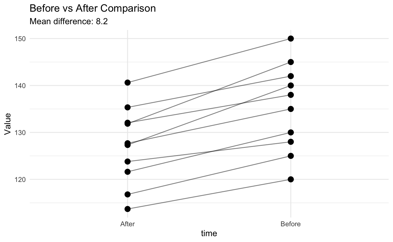

Exercise 3:

safe_t_test <- function(x, y = NULL, paired = FALSE, ...) {
  
  # Check inputs
  if (is.null(y)) {
    # One-sample test
    if (length(x) < 2) {
      stop("Need at least 2 observations")
    }
    if (sd(x) == 0) {
      stop("Data has no variation")
    }
  } else {
    # Two-sample test
    if (length(x) < 2) stop("x needs at least 2 observations")
    if (length(y) < 2) stop("y needs at least 2 observations")
    if (sd(x) == 0) stop("x has no variation")
    if (sd(y) == 0) stop("y has no variation")
    
    # Check paired
    if (paired && length(x) != length(y)) {
      stop("For paired test, x and y must have same length")
    }
  }
  
  # Perform test
  result <- t.test(x, y, paired = paired, ...)
  
  # Format output
  output <- list(
    test = result,
    summary = data.frame(
      statistic = result$statistic,
      df = result$parameter,
      p_value = result$p.value,
      mean_diff = ifelse(is.null(y), 
                         result$estimate - result$null.value,
                         diff(result$estimate)),
      ci_lower = result$conf.int[1],
      ci_upper = result$conf.int[2]
    )
  )
  
  # Print summary
  cat("=== t-test Results ===\n")
  cat("t =", round(output$summary$statistic, 3), "\n")
  cat("df =", round(output$summary$df, 1), "\n")
  cat("p-value =", format.pval(output$summary$p_value, digits = 3), "\n")
  cat("Mean difference =", round(output$summary$mean_diff, 2), "\n")
  cat("95% CI: [", round(output$summary$ci_lower, 2), ",",
      round(output$summary$ci_upper, 2), "]\n")
  
  if (output$summary$p_value < 0.05) {
    cat("\nSignificant at α = 0.05\n")
  } else {
    cat("\nNot significant at α = 0.05\n")
  }
  
  invisible(output)
}

# Test it
safe_t_test(mtcars$mpg[mtcars$am == 0], mtcars$mpg[mtcars$am == 1])
#> === t-test Results ===
#> t = -3.767 
#> df = 18.3 
#> p-value = 0.00137 
#> Mean difference = 7.24 
#> 95% CI: [ -11.28 , -3.21 ]
#> 
#> Significant at α = 0.05

Exercise 4:

library(dplyr)

# 1 & 2. All pairwise comparisons
species <- levels(iris$Species)
results_list <- list()

for (i in 1:(length(species) - 1)) {
  for (j in (i + 1):length(species)) {
    sp1 <- species[i]
    sp2 <- species[j]
    
    data_subset <- iris %>%
      filter(Species %in% c(sp1, sp2))
    
    test <- t.test(Petal.Length ~ Species, data = data_subset)
    
    results_list[[paste(sp1, "vs", sp2)]] <- data.frame(
      comparison = paste(sp1, "vs", sp2),
      mean_1 = test$estimate[1],
      mean_2 = test$estimate[2],
      mean_diff = diff(test$estimate),
      t_stat = test$statistic,
      p_value = test$p.value,
      ci_lower = test$conf.int[1],
      ci_upper = test$conf.int[2]
    )
  }
}

results_df <- do.call(rbind, results_list)
rownames(results_df) <- NULL

# 3. Adjust for multiple testing
results_df$p_adjusted <- p.adjust(results_df$p_value, method = "bonferroni")

# 4. Display results
cat("=== Pairwise Comparisons of Petal Length ===\n\n")
#> === Pairwise Comparisons of Petal Length ===
print(results_df, digits = 3)
#>                comparison mean_1 mean_2 mean_diff t_stat  p_value ci_lower
#> 1    setosa vs versicolor   1.46   4.26      2.80  -39.5 9.93e-46    -2.94
#> 2     setosa vs virginica   1.46   5.55      4.09  -50.0 9.27e-50    -4.25
#> 3 versicolor vs virginica   4.26   5.55      1.29  -12.6 4.90e-22    -1.50
#>   ci_upper p_adjusted
#> 1    -2.66   2.98e-45
#> 2    -3.93   2.78e-49
#> 3    -1.09   1.47e-21

cat("\n=== Summary ===\n")
#> 
#> === Summary ===
cat("Total comparisons:", nrow(results_df), "\n")
#> Total comparisons: 3
cat("Significant (unadjusted):", sum(results_df$p_value < 0.05), "\n")
#> Significant (unadjusted): 3
cat("Significant (Bonferroni):", sum(results_df$p_adjusted < 0.05), "\n")
#> Significant (Bonferroni): 3

Chapter 30 Statistical Tests

30.1 Introduction

30.2 t-tests

30.3 Error #1: not enough 'x' observations

30.3.1 The Error

30.3.2 What It Means

30.3.3 Common Causes

30.3.4 Solutions

30.4 Error #2: data are essentially constant

30.4.1 The Error

30.4.2 What It Means

30.4.3 Common Causes

30.4.4 Solutions

30.5 Formula Interface

30.6 Error #3: grouping factor must have 2 levels

30.6.1 The Error

30.6.2 What It Means

30.6.3 Solutions

30.7 Assumptions

30.8 Interpreting Results

30.9 Effect Size

30.10 Paired t-tests

30.11 Error #4: 'x' and 'y' must have the same length

30.11.1 The Error

30.11.2 What It Means

30.11.3 Solutions

30.12 Power and Sample Size

30.13 Summary

30.14 Exercises

30.15 Exercise Answers

30.3 Error #1: `not enough 'x' observations`

30.4 Error #2: `data are essentially constant`

30.6 Error #3: `grouping factor must have 2 levels`

30.11 Error #4: `'x' and 'y' must have the same length`