Chapter 26 Introduction to ggplot2
What You’ll Learn:
- Grammar of Graphics principles
- Basic ggplot2 structure
- Common plotting errors
- Aesthetics and geoms
- Layer system
Key Errors Covered: 20+ ggplot2 errors
Difficulty: ⭐⭐ Intermediate to ⭐⭐⭐ Advanced
26.1 Introduction
ggplot2 revolutionized R graphics with the Grammar of Graphics:

But ggplot2 has unique error patterns. Let’s master them!
26.2 ggplot2 Structure
💡 Key Insight: Grammar of Graphics
# Three essential components:
# 1. Data
# 2. Aesthetic mappings (aes)
# 3. Geometric objects (geom)
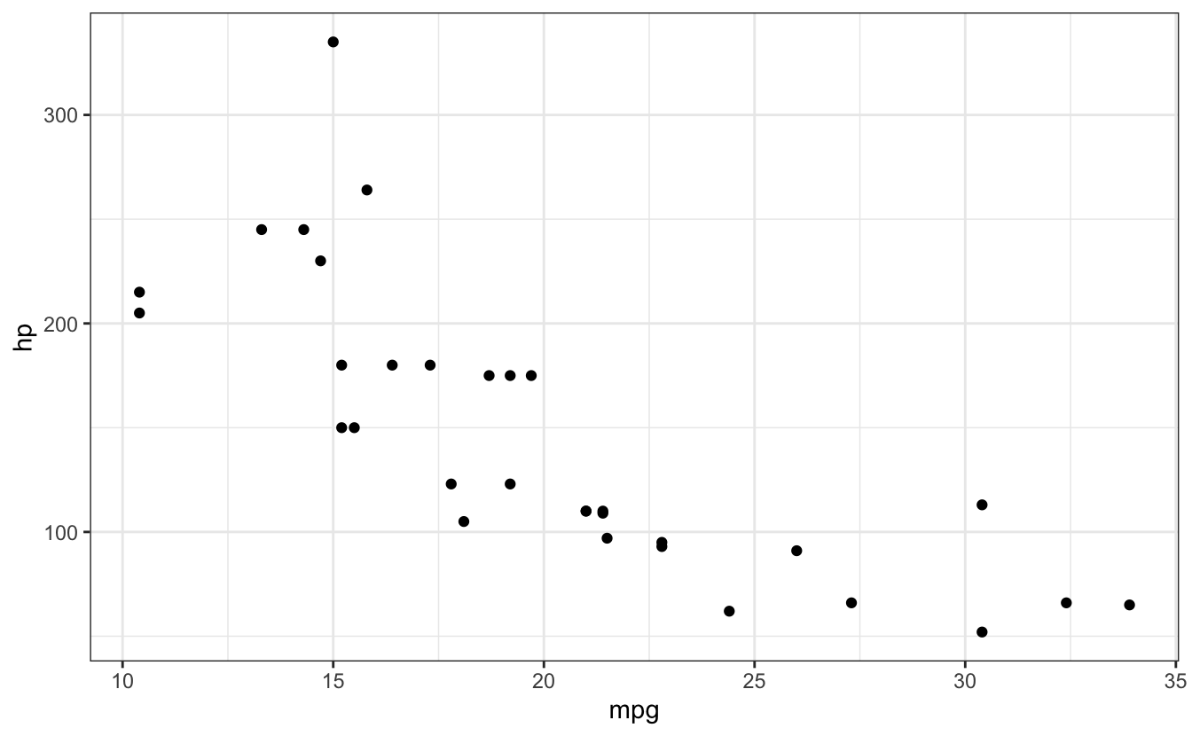
# Basic structure
ggplot(data = mtcars, mapping = aes(x = mpg, y = hp)) +
geom_point()
# Shortened (common)
ggplot(mtcars, aes(x = mpg, y = hp)) +
geom_point()
# Can specify aes in geom instead
ggplot(mtcars) +
geom_point(aes(x = mpg, y = hp))
# Or mix (useful for multiple layers)
ggplot(mtcars, aes(x = mpg, y = hp)) +
geom_point() +
geom_smooth()
#> `geom_smooth()` using method = 'loess' and formula = 'y ~ x'


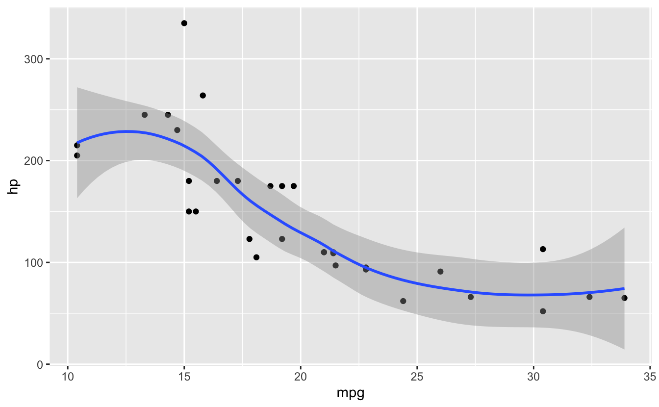
Key principle: Build plots in layers with +
26.3 Error #1: object not found in aes()
⭐ BEGINNER 🔍 SCOPE
26.3.1 The Error
ggplot(mtcars, aes(x = mpg, y = horsepower)) +
  geom_point()
#> Error in `geom_point()`:
#> ! Problem while computing aesthetics.
#> ℹ Error occurred in the 1st layer.
#> Caused by error:
#> ! object 'horsepower' not found
🔴 ERROR
Error in FUN(X[[i]], ...) : object 'horsepower' not found26.3.3 Common Causes
# Typo in column name
ggplot(mtcars, aes(x = mpgg, y = hp)) +
geom_point()
#> Error in `geom_point()`:
#> ! Problem while computing aesthetics.
#> ℹ Error occurred in the 1st layer.
#> Caused by error:
#> ! object 'mpgg' not found
# Wrong dataset
ggplot(iris, aes(x = mpg, y = hp)) +
geom_point()
#> Error in `geom_point()`:
#> ! Problem while computing aesthetics.
#> ℹ Error occurred in the 1st layer.
#> Caused by error:
#> ! object 'hp' not found
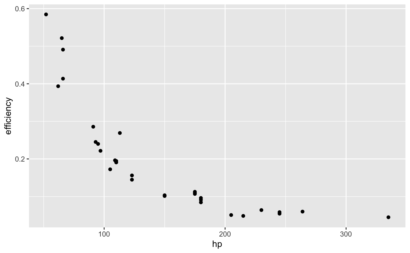
# Forgot to create column
ggplot(mtcars, aes(x = mpg, y = efficiency)) +
geom_point()
#> Error in `geom_point()`:
#> ! Problem while computing aesthetics.
#> ℹ Error occurred in the 1st layer.
#> Caused by error:
#> ! object 'efficiency' not found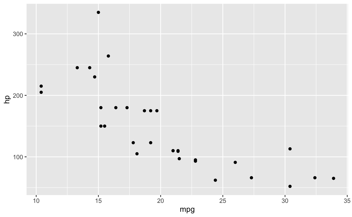
26.4 Error #2: Using + vs %>%
⭐ BEGINNER 🔤 SYNTAX
26.4.1 The Error
library(dplyr)

mtcars %>%
  filter(cyl == 4) %>%
  ggplot(aes(x = mpg, y = hp)) %>%  # Wrong operator!
  geom_point()
#> Error in `geom_point()`:
#> ! `mapping` must be created by `aes()`.
#> ✖ You've supplied a <ggplot2::ggplot> object.
#> ℹ Did you use `%>%` or `|>` instead of `+`?
🔴 ERROR
Error in geom_point(.) :
  Cannot use `+` with a ggplot object. Did you accidentally use `%>%` instead of `+`?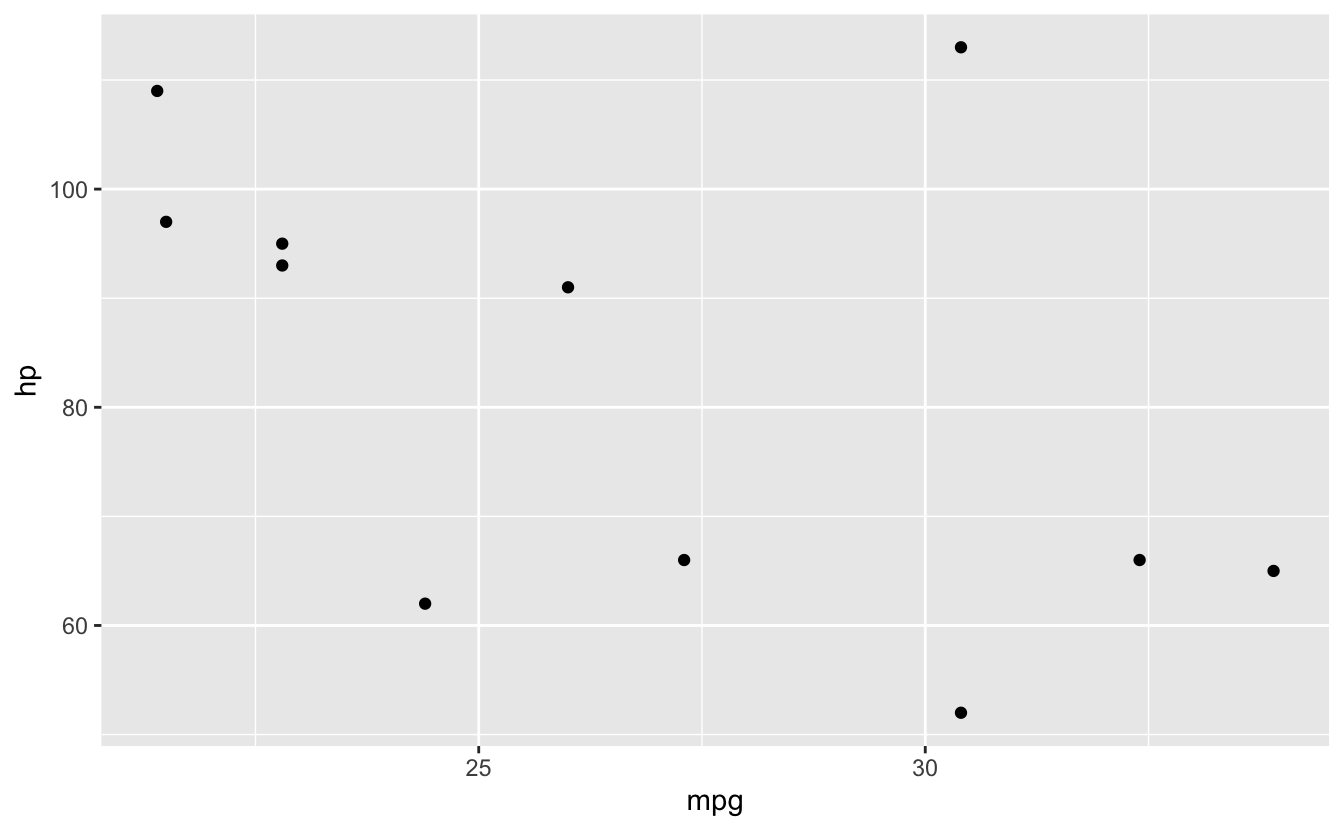
26.5 Aesthetics (aes)
💡 Key Insight: Aesthetic Mappings
# Map variables to visual properties
ggplot(mtcars, aes(x = mpg, y = hp, color = factor(cyl))) +
geom_point()
# Common aesthetics:
# x, y - position
# color - point/line color
# fill - area fill color
# size - point/line size
# shape - point shape
# alpha - transparency
# linetype - line pattern
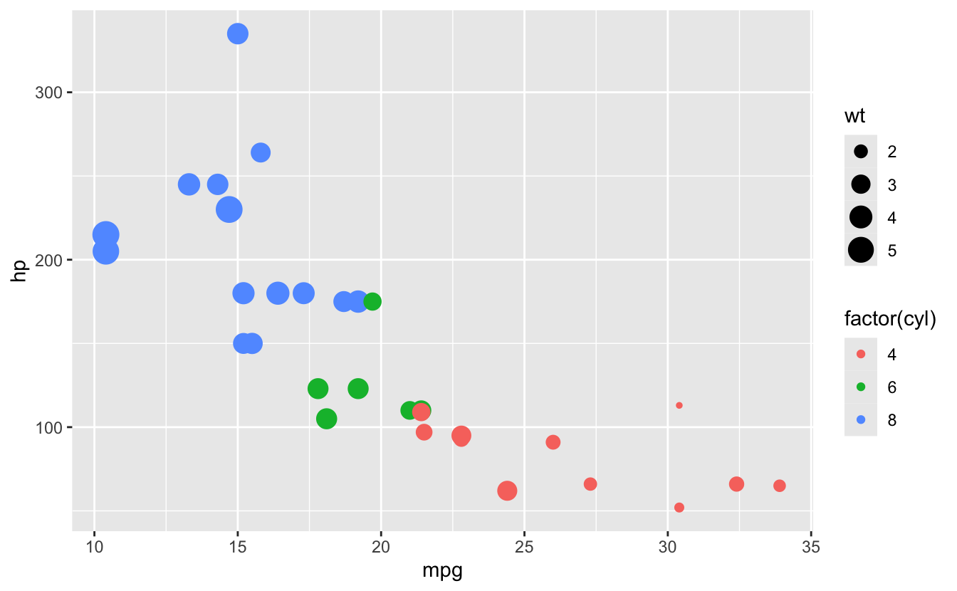
# Multiple aesthetics
ggplot(mtcars, aes(x = mpg, y = hp,
color = factor(cyl),
size = wt)) +
geom_point()
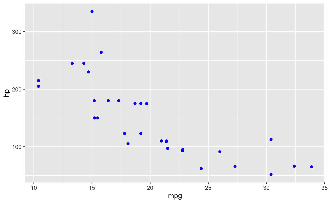
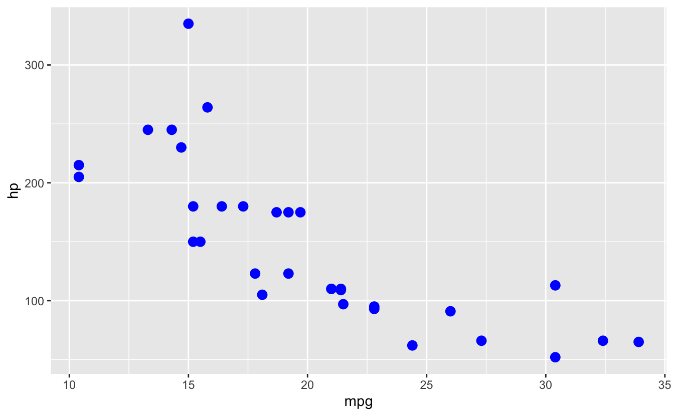
# Set vs map
ggplot(mtcars, aes(x = mpg, y = hp)) +
geom_point(color = "blue") # Set: all points blue
ggplot(mtcars, aes(x = mpg, y = hp, color = factor(cyl))) +
geom_point() # Map: color varies by cyl

26.6 Error #3: Aesthetic outside aes()
⭐⭐ INTERMEDIATE 🧠 LOGIC
26.6.1 The Error
# Trying to map cyl to color outside aes()
ggplot(mtcars) +
  geom_point(aes(x = mpg, y = hp), color = cyl)
#> Error: object 'cyl' not found
🔴 ERROR
Error in layer(...) : object 'cyl' not found26.6.4 Solutions
✅ SOLUTION: Put Variable Mappings in aes()
# Correct: color mapping inside aes
ggplot(mtcars) +
  geom_point(aes(x = mpg, y = hp, color = factor(cyl)))

# Can be in ggplot() aes
ggplot(mtcars, aes(x = mpg, y = hp, color = factor(cyl))) +
  geom_point()

# Fixed values go OUTSIDE aes
ggplot(mtcars, aes(x = mpg, y = hp)) +
  geom_point(color = "blue", size = 3)  # All points same

⚠️ Common Confusion: Inside vs Outside aes()
# INSIDE aes(): varies by data
ggplot(mtcars, aes(x = mpg, y = hp, color = factor(cyl))) +
geom_point() # Color varies by cyl
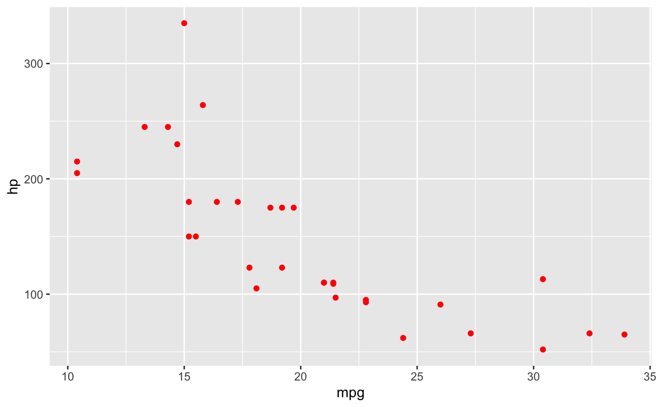
# OUTSIDE aes(): fixed for all
ggplot(mtcars, aes(x = mpg, y = hp)) +
geom_point(color = "red") # All points red
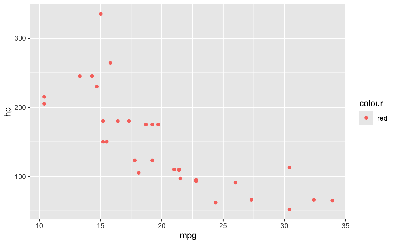
# Wrong: puts string in aes
ggplot(mtcars, aes(x = mpg, y = hp, color = "red")) +
geom_point() # Creates legend for "red"!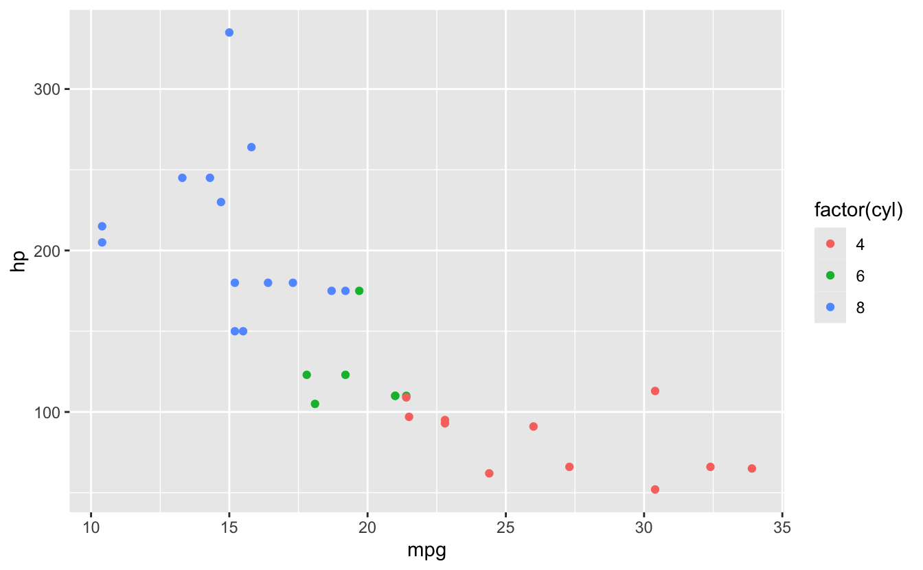
26.7 Common geoms
💡 Key Insight: Geometric Objects
# Points
ggplot(mtcars, aes(x = mpg, y = hp)) +
geom_point()
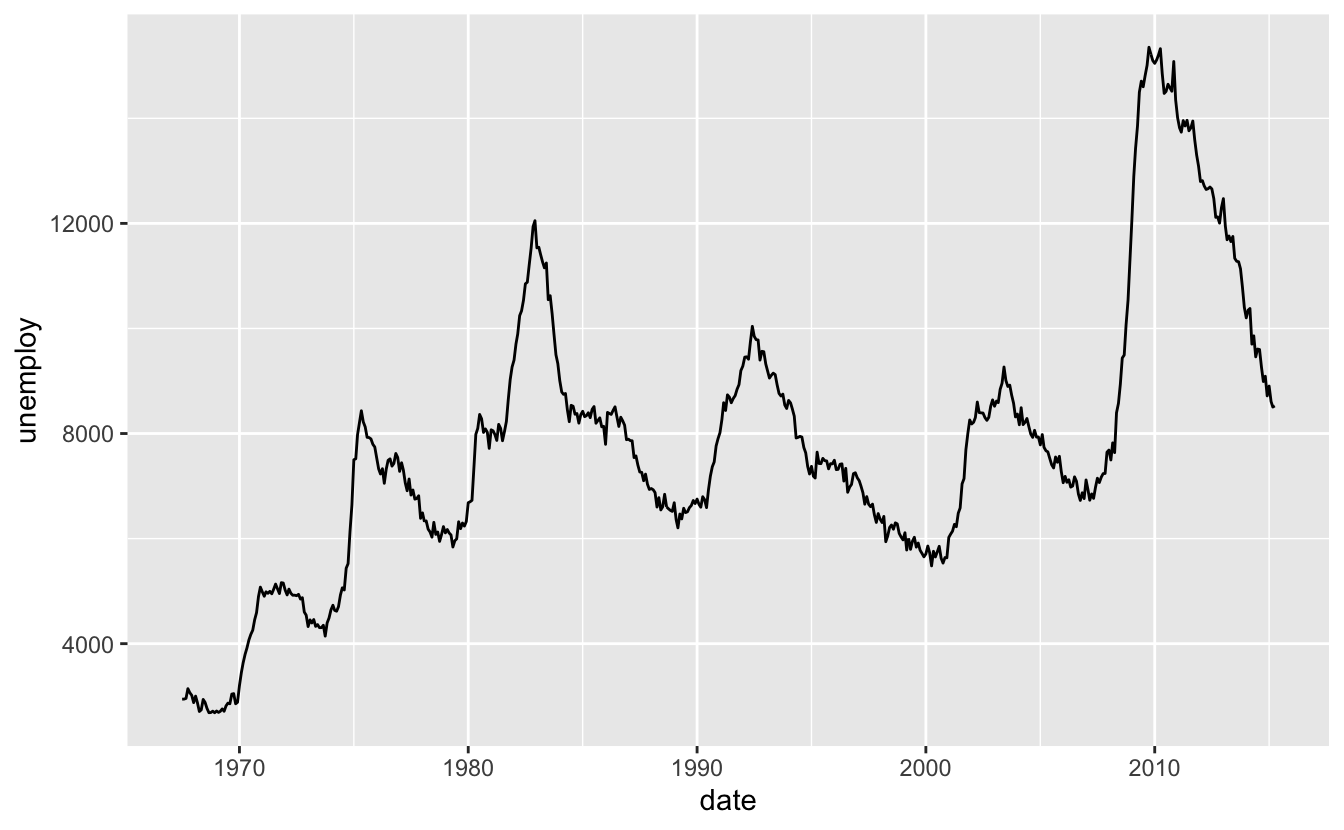
# Lines
ggplot(economics, aes(x = date, y = unemploy)) +
geom_line()
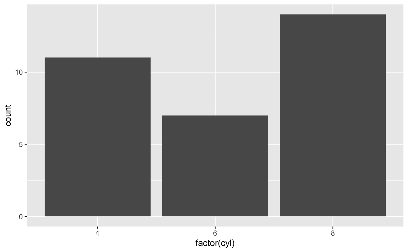
# Bars
ggplot(mtcars, aes(x = factor(cyl))) +
geom_bar()
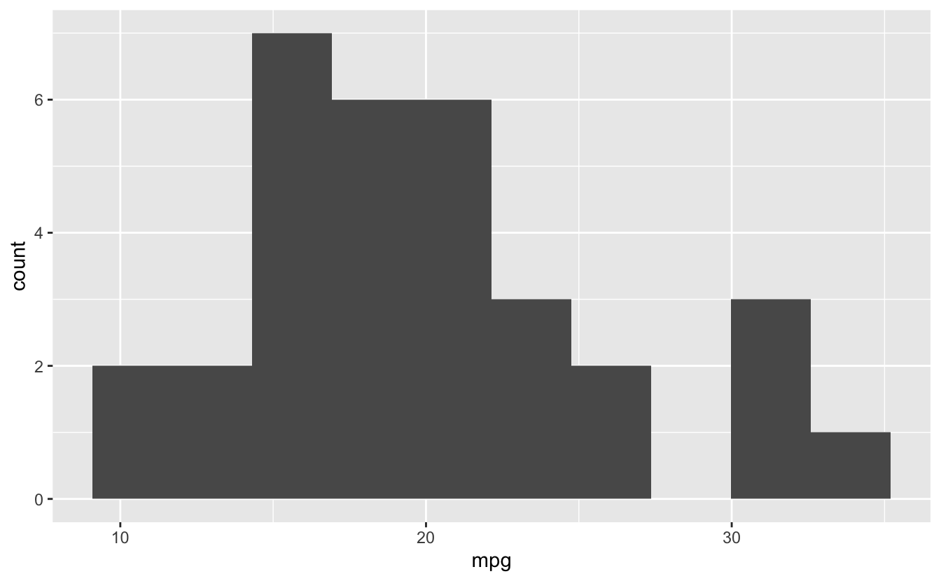
# Histogram
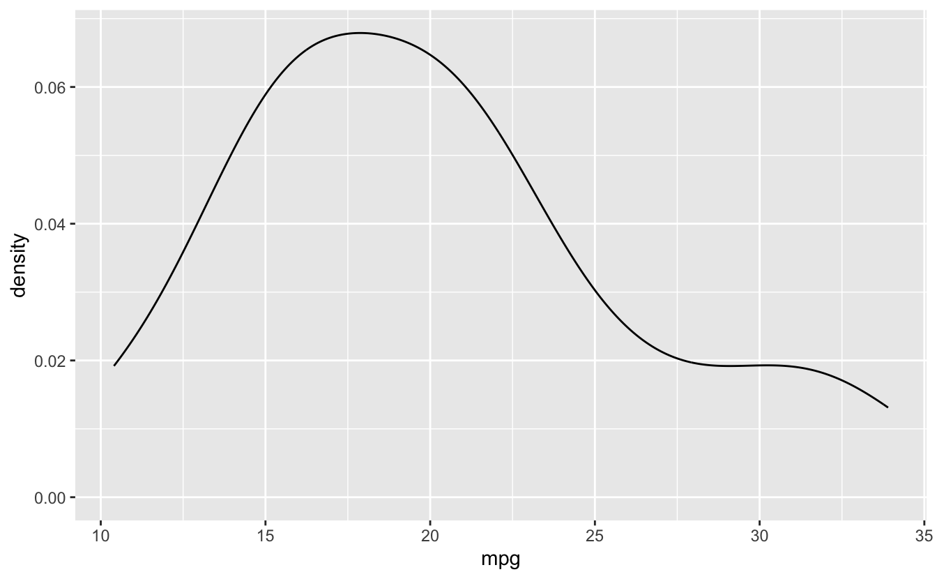
ggplot(mtcars, aes(x = mpg)) +
geom_histogram(bins = 10)
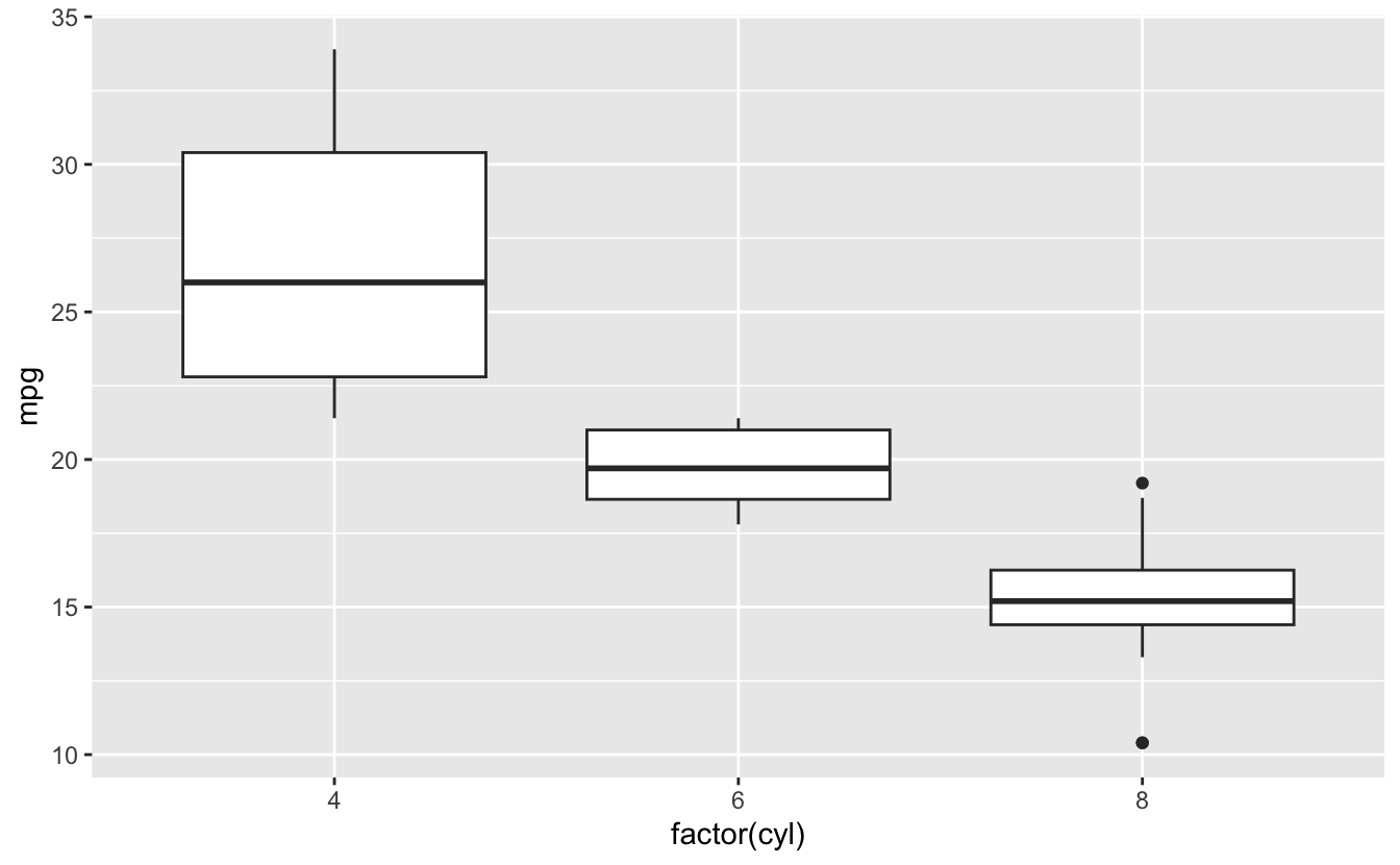
# Boxplot
ggplot(mtcars, aes(x = factor(cyl), y = mpg)) +
geom_boxplot()
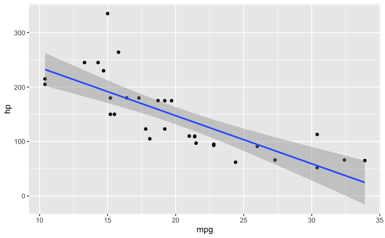
# Smooth
ggplot(mtcars, aes(x = mpg, y = hp)) +
geom_point() +
geom_smooth(method = "lm")
#> `geom_smooth()` using formula = 'y ~ x'
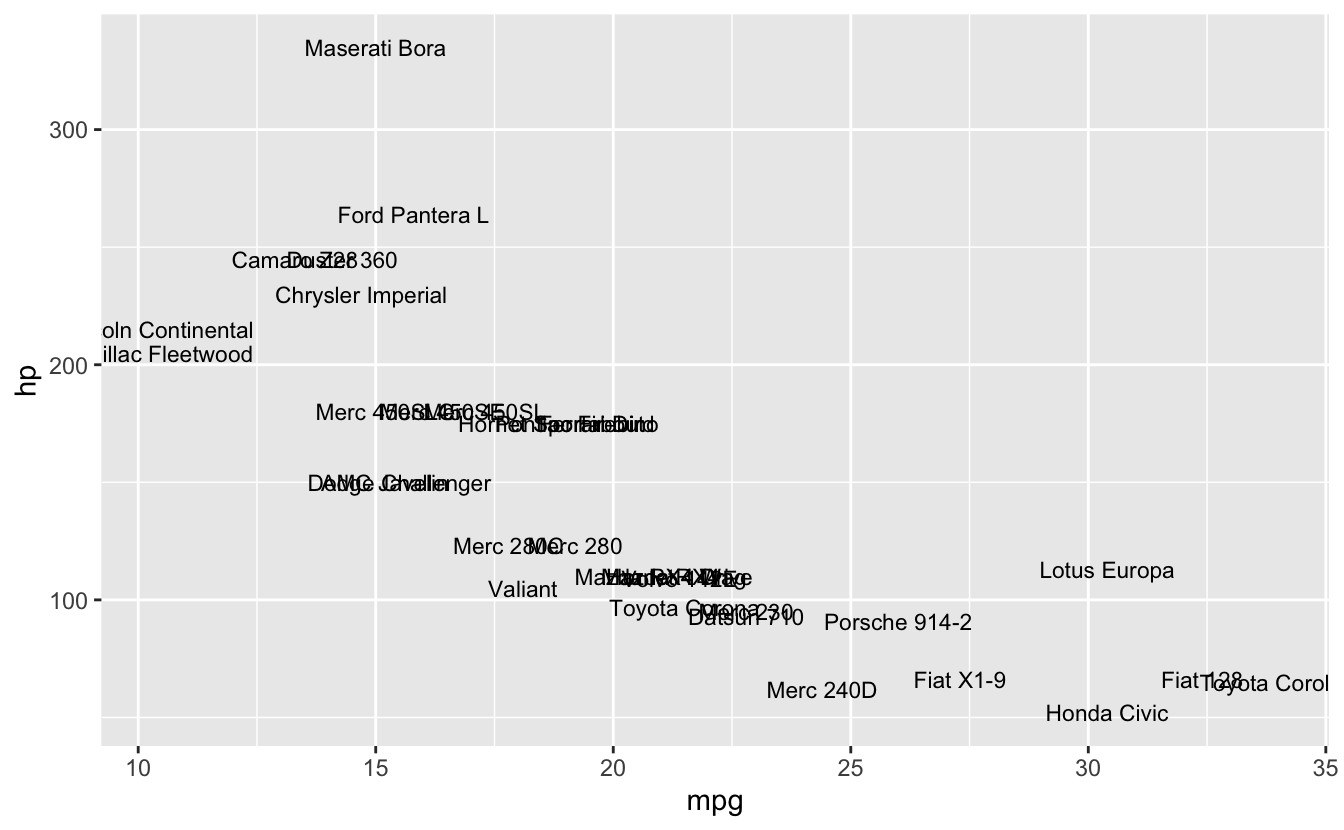
# Text
ggplot(mtcars, aes(x = mpg, y = hp, label = rownames(mtcars))) +
geom_text(size = 3)


26.8 Error #4: stat_count() requires x or y
⭐ BEGINNER 📋 ARGS
26.8.1 The Error
ggplot(mtcars, aes(x = mpg, y = hp)) +
  geom_bar()
#> Error in `geom_bar()`:
#> ! Problem while computing stat.
#> ℹ Error occurred in the 1st layer.
#> Caused by error in `setup_params()`:
#> ! `stat_count()` must only have an x or y aesthetic.
🔴 ERROR
Error in `geom_bar()`:
! Problem while computing stat.
ℹ Error occurred in the 1st layer.
Caused by error:
! `stat_count()` must only have an `x` or `y` aesthetic.26.8.3 Solutions
✅ SOLUTION 1: Use geom_col() for Heights
# Pre-computed values
data <- data.frame(
  category = c("A", "B", "C"),
  value = c(10, 15, 20)
)

ggplot(data, aes(x = category, y = value)) +
  geom_col()

# Or use stat = "identity" with geom_bar
ggplot(data, aes(x = category, y = value)) +
  geom_bar(stat = "identity")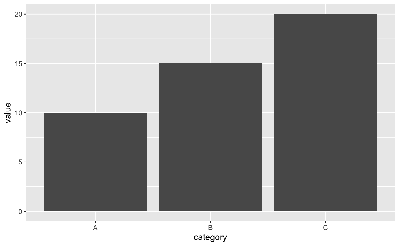


26.9 Faceting
💡 Key Insight: Small Multiples
# Facet by one variable
ggplot(mtcars, aes(x = mpg, y = hp)) +
geom_point() +
facet_wrap(~ cyl)
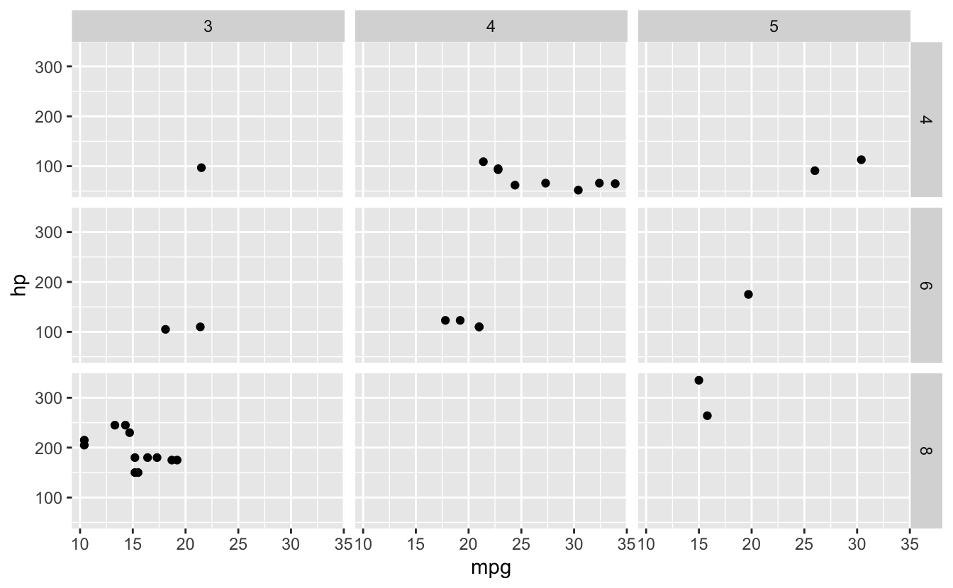
# Facet by two variables
ggplot(mtcars, aes(x = mpg, y = hp)) +
geom_point() +
facet_grid(cyl ~ gear)
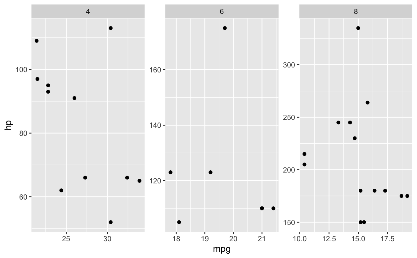
# Free scales
ggplot(mtcars, aes(x = mpg, y = hp)) +
geom_point() +
facet_wrap(~ cyl, scales = "free")
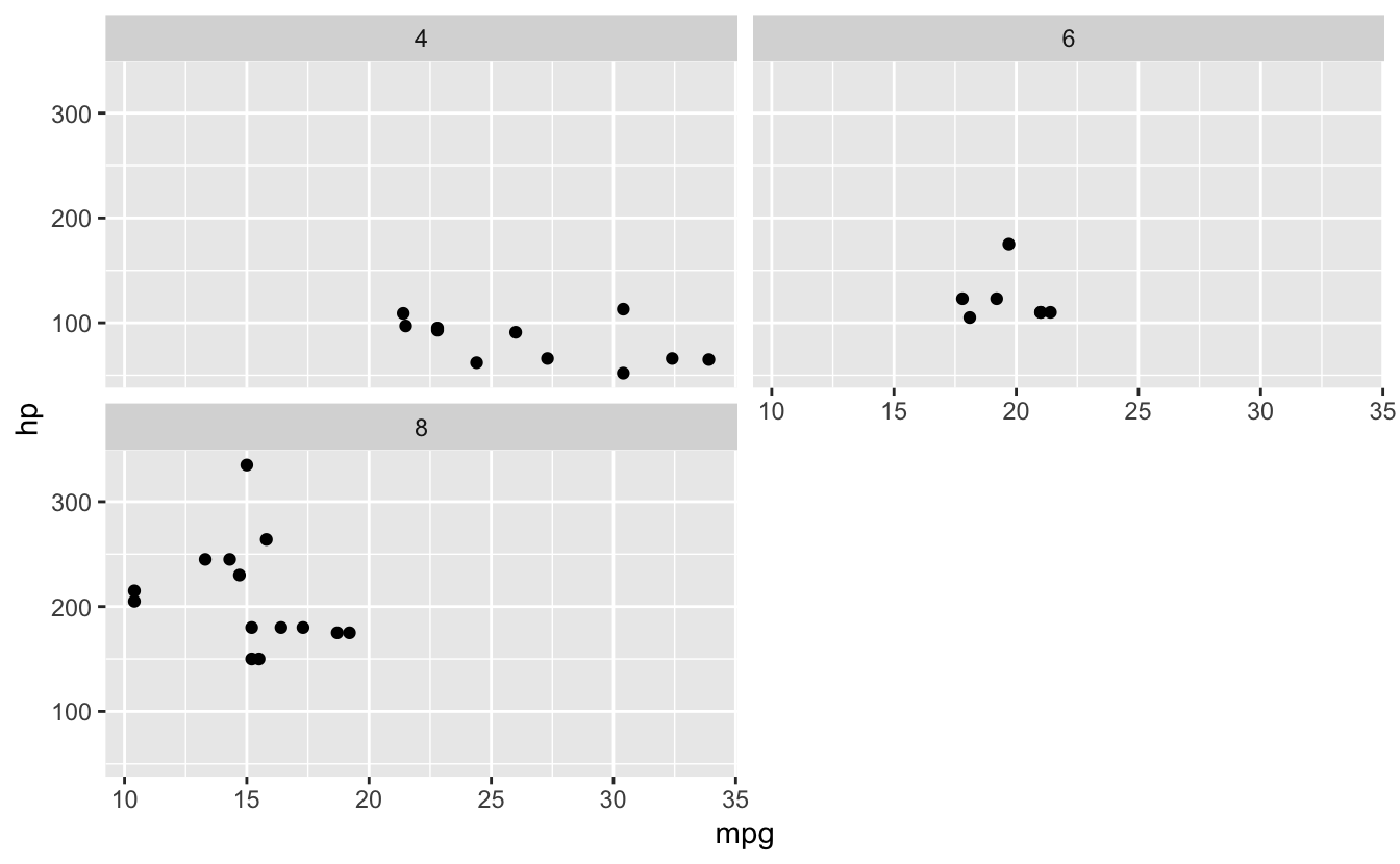
# Number of columns
ggplot(mtcars, aes(x = mpg, y = hp)) +
geom_point() +
facet_wrap(~ cyl, ncol = 2)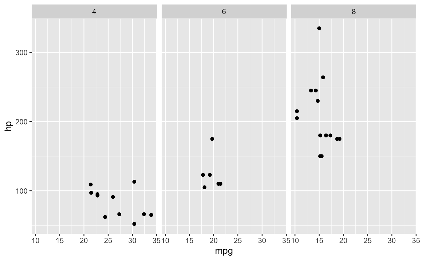
26.10 Themes and Customization
🎯 Best Practice: Customizing Plots
# Built-in themes
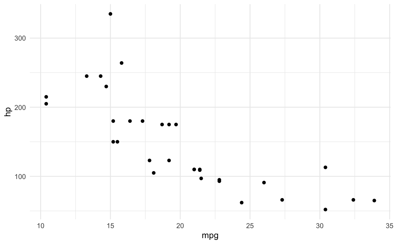
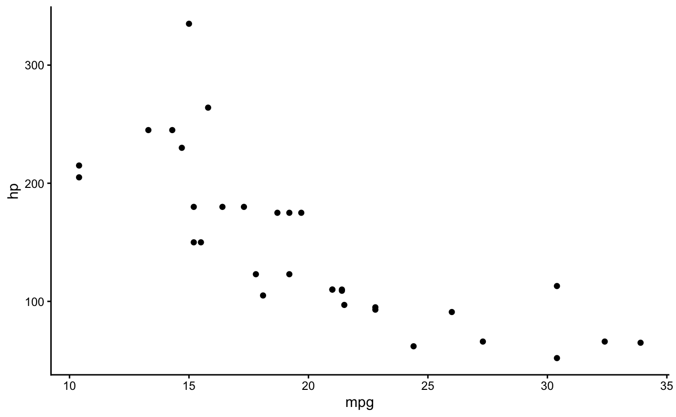
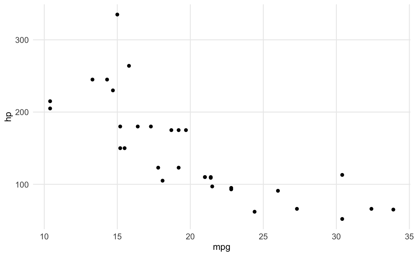
p <- ggplot(mtcars, aes(x = mpg, y = hp)) +
geom_point()
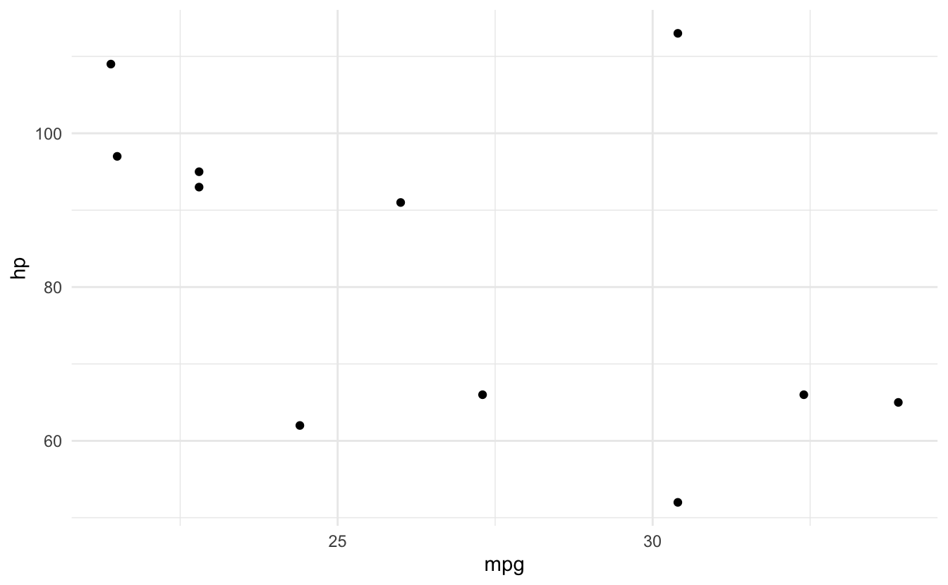
p + theme_minimal()
p + theme_classic()
p + theme_bw()
# Custom labels
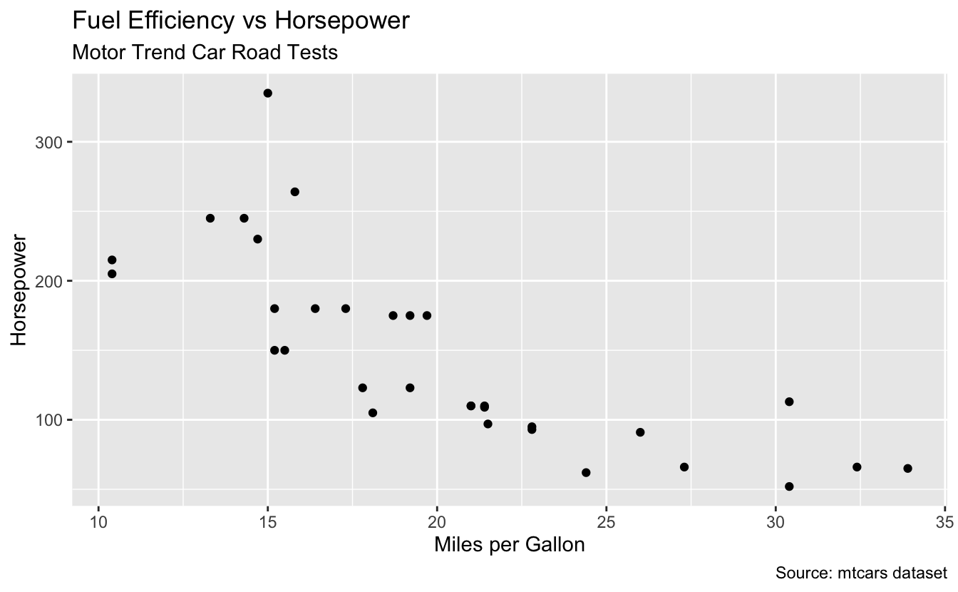
ggplot(mtcars, aes(x = mpg, y = hp)) +
geom_point() +
labs(
title = "Fuel Efficiency vs Horsepower",
subtitle = "Motor Trend Car Road Tests",
x = "Miles per Gallon",
y = "Horsepower",
caption = "Source: mtcars dataset"
)
# Customize theme elements
ggplot(mtcars, aes(x = mpg, y = hp)) +
geom_point() +
theme_minimal() +
theme(
plot.title = element_text(face = "bold", size = 14),
axis.text = element_text(size = 10),
panel.grid.minor = element_blank()
)
26.11 Error #5: Non-numeric variable for histogram
⭐ BEGINNER 🔢 TYPE
26.11.1 The Error
ggplot(mtcars, aes(x = factor(cyl))) +
  geom_histogram()
#> Error in `geom_histogram()`:
#> ! Problem while computing stat.
#> ℹ Error occurred in the 1st layer.
#> Caused by error in `setup_params()`:
#> ! `stat_bin()` requires a continuous x aesthetic.
#> ✖ the x aesthetic is discrete.
#> ℹ Perhaps you want `stat="count"`?
🔴 ERROR
Error in `geom_histogram()`:
! `stat_bin()` requires a numeric `x` variable

26.12 Saving Plots
🎯 Best Practice: Save Plots
# Create plot
p <- ggplot(mtcars, aes(x = mpg, y = hp)) +
  geom_point() +
  theme_minimal()

# Save with ggsave
ggsave("plot.png", p, width = 6, height = 4, dpi = 300)

# Or save last plot
ggplot(mtcars, aes(x = mpg, y = hp)) +
  geom_point()

ggsave("last_plot.png", width = 6, height = 4)

# Different formats
ggsave("plot.pdf", p)
ggsave("plot.svg", p)
ggsave("plot.jpg", p)
26.13 Common Patterns
🎯 Best Practice: Common Plot Types
# Scatterplot with trend line
ggplot(mtcars, aes(x = mpg, y = hp)) +
geom_point(aes(color = factor(cyl))) +
geom_smooth(method = "lm", se = FALSE) +
theme_minimal()
#> `geom_smooth()` using formula = 'y ~ x'
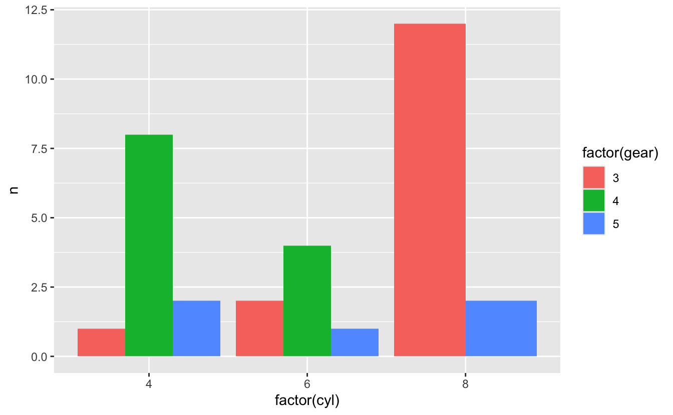
# Grouped bar chart
mtcars %>%
count(cyl, gear) %>%
ggplot(aes(x = factor(cyl), y = n, fill = factor(gear))) +
geom_col(position = "dodge")
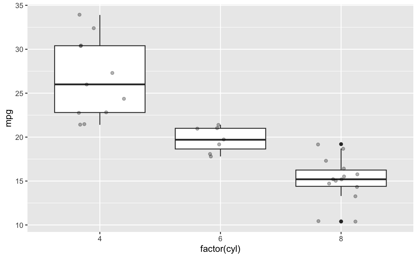
# Boxplot with points
ggplot(mtcars, aes(x = factor(cyl), y = mpg)) +
geom_boxplot() +
geom_jitter(width = 0.2, alpha = 0.3)
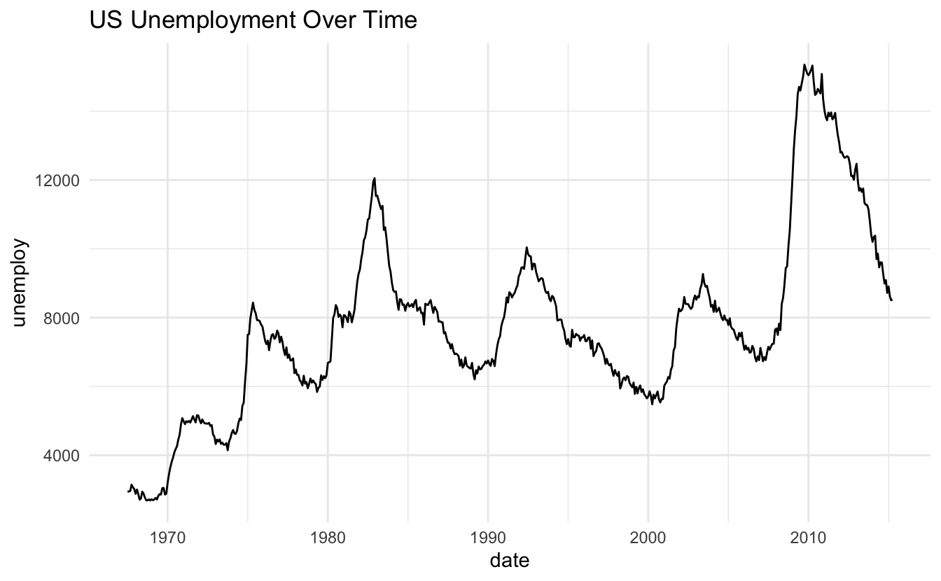
# Time series
ggplot(economics, aes(x = date, y = unemploy)) +
geom_line() +
theme_minimal() +
labs(title = "US Unemployment Over Time")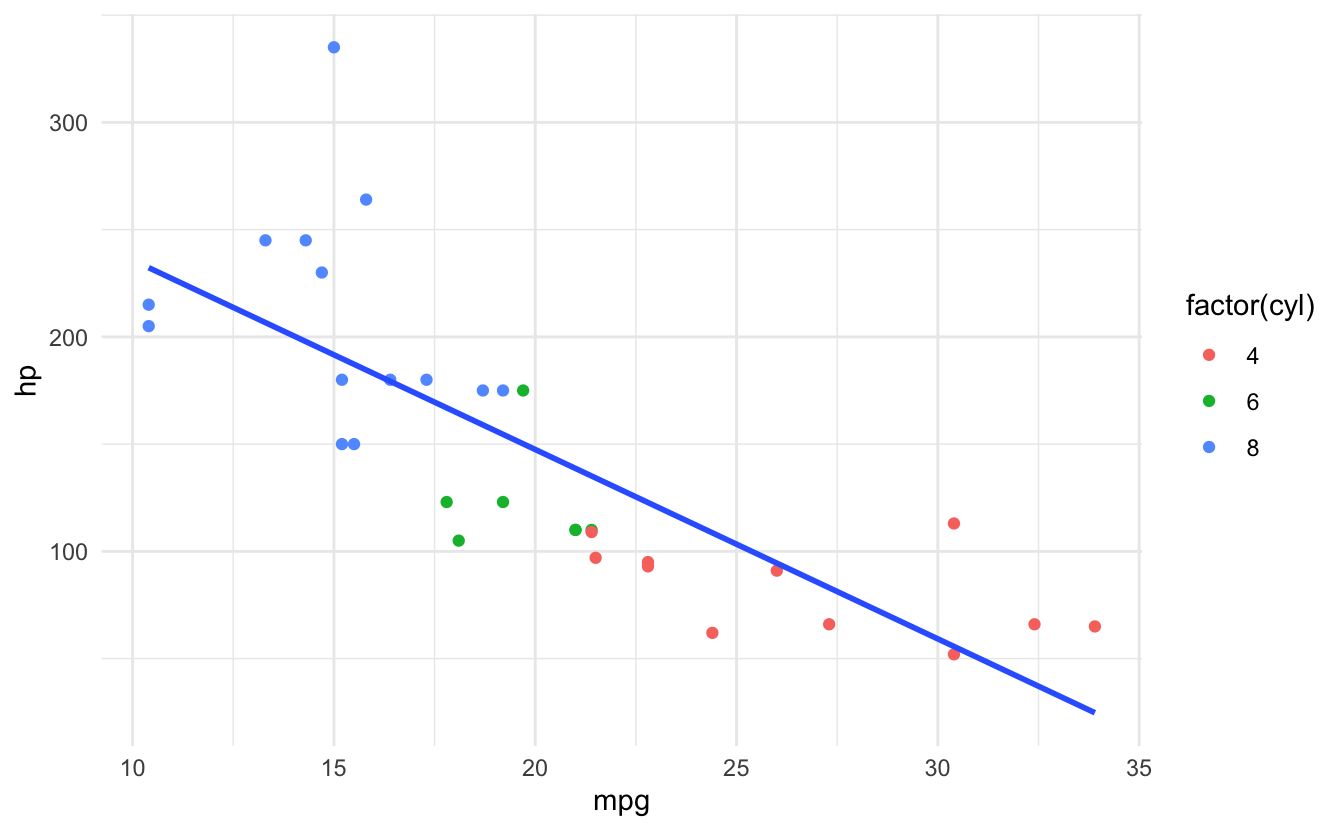
26.14 Summary
Key Takeaways:
- Three components - Data, aes(), geom
- Use + not %>% - Add layers with +
- Variables in aes() - Fixed values outside
- geom_bar() vs geom_col() - Counts vs heights
- Check column names - Before plotting
- Histograms need numeric - Use geom_bar() for categorical
- Build in layers - Add components step by step
Quick Reference:
| Error | Cause | Fix |
|---|---|---|
| object not found | Column doesn’t exist | Check names(data) |
| Can’t use + | Used %>% instead of + | Use + for ggplot layers |
| object ‘var’ not found | Variable outside aes | Put in aes() |
| stat_count requires x or y | geom_bar with y | Use geom_col() |
| requires numeric x | Non-numeric histogram | Use appropriate geom |
Basic Structure:
# Template
ggplot(data, aes(x = var1, y = var2)) +
  geom_point() +
  theme_minimal()

# With pipes
data %>%
  filter(condition) %>%
  ggplot(aes(x = var1, y = var2)) +  # Use +
  geom_point() +
  labs(title = "Plot Title")

# Common aesthetics
aes(
  x = var,           # x-axis
  y = var,           # y-axis
  color = var,       # point/line color
  fill = var,        # area fill
  size = var,        # size
  shape = var,       # point shape
  alpha = var,       # transparency
  linetype = var     # line pattern
)

# Common geoms
geom_point()         # scatter
geom_line()          # line
geom_bar()           # bar (counts)
geom_col()           # bar (heights)
geom_histogram()     # histogram
geom_boxplot()       # boxplot
geom_smooth()        # trend line
Best Practices:
# ✅ Good
ggplot(data, aes(x = var1, y = var2, color = var3)) +
  geom_point() +
  theme_minimal()

data %>% filter(...) %>%
  ggplot(aes(x = var)) +  # + not %>%
  geom_histogram()

# ❌ Avoid
ggplot(data, aes(x = var1, y = var2)) %>%  # Wrong operator
  geom_point()

ggplot(data) +
  geom_point(aes(x = var), color = other_var)  # Should be in aes

geom_histogram(aes(x = factor_var))  # Need numeric
26.15 Exercises
📝 Exercise 1: Basic Plot
Create a scatterplot of mtcars: 1. mpg vs hp 2. Color by cyl 3. Size by wt 4. Add title and labels 5. Use theme_minimal()
📝 Exercise 2: Error Fixing
Fix these errors:
📝 Exercise 3: Multiple Geoms
Create a plot with: 1. Points for raw data 2. Smooth line for trend 3. Faceted by cyl 4. Custom colors
📝 Exercise 4: Bar Chart
Using mtcars: 1. Count cars by cyl 2. Fill by gear 3. Dodge position 4. Add labels
26.16 Exercise Answers
Click to see answers
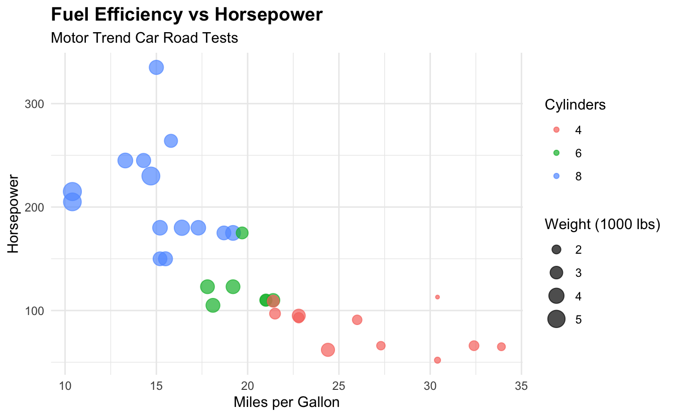
Exercise 1:
ggplot(mtcars, aes(x = mpg, y = hp, color = factor(cyl), size = wt)) +
  geom_point(alpha = 0.7) +
  labs(
    title = "Fuel Efficiency vs Horsepower",
    subtitle = "Motor Trend Car Road Tests",
    x = "Miles per Gallon",
    y = "Horsepower",
    color = "Cylinders",
    size = "Weight (1000 lbs)"
  ) +
  theme_minimal() +
  theme(
    plot.title = element_text(face = "bold", size = 14),
    legend.position = "right"
  )
Exercise 2:
# Error 1: Use + not %>%
ggplot(mtcars, aes(x = mpg, y = hp)) +
  geom_point()

# Error 2: Put variable in aes()
ggplot(mtcars) +
  geom_point(aes(x = mpg, y = hp, color = factor(cyl)))

# Error 3: Use geom_boxplot for this
ggplot(mtcars, aes(x = factor(cyl), y = mpg)) +
  geom_boxplot()

# Or if want histogram of mpg
ggplot(mtcars, aes(x = mpg)) +
  geom_histogram(bins = 10)


Exercise 3:
ggplot(mtcars, aes(x = mpg, y = hp)) +
  geom_point(aes(color = factor(cyl)), size = 3, alpha = 0.6) +
  geom_smooth(method = "lm", se = FALSE, color = "black", linetype = "dashed") +
  facet_wrap(~ cyl, labeller = label_both) +
  scale_color_manual(values = c("4" = "#E41A1C", "6" = "#377EB8", "8" = "#4DAF4A")) +
  labs(
    title = "MPG vs HP by Number of Cylinders",
    x = "Miles per Gallon",
    y = "Horsepower",
    color = "Cylinders"
  ) +
  theme_bw()
#> `geom_smooth()` using formula = 'y ~ x'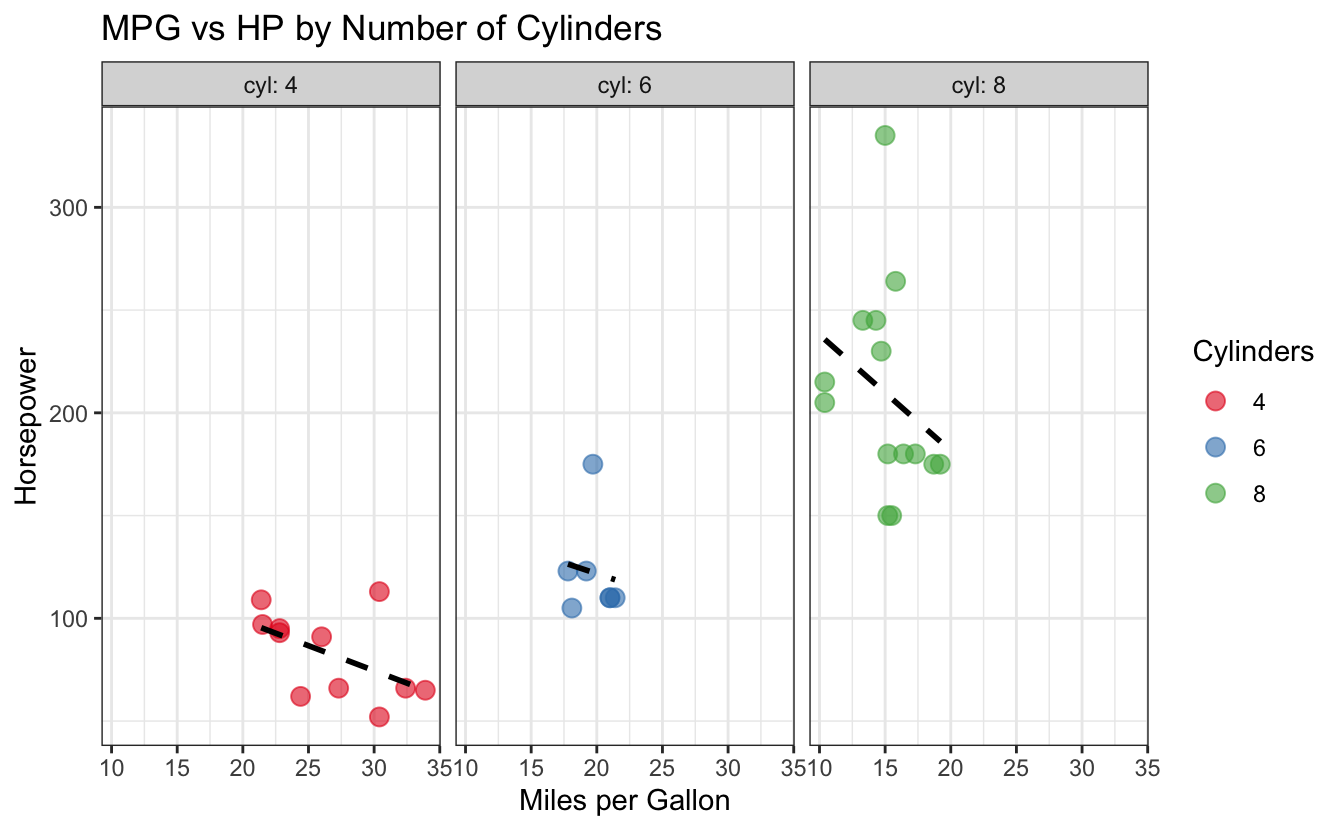
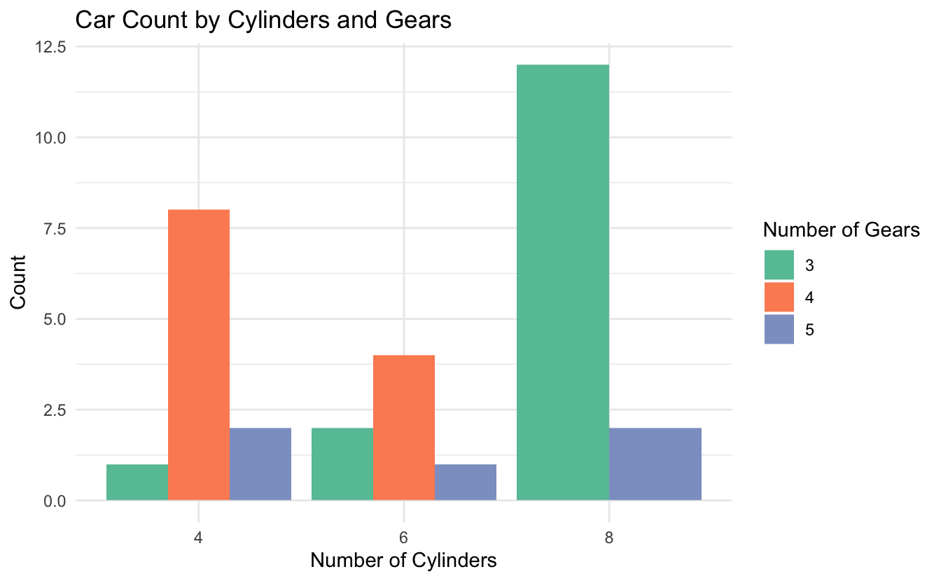
Exercise 4:
library(dplyr)

mtcars %>%
  count(cyl, gear) %>%
  ggplot(aes(x = factor(cyl), y = n, fill = factor(gear))) +
  geom_col(position = "dodge") +
  labs(
    title = "Car Count by Cylinders and Gears",
    x = "Number of Cylinders",
    y = "Count",
    fill = "Number of Gears"
  ) +
  theme_minimal() +
  scale_fill_brewer(palette = "Set2")