Chapter 5 Prognostic modeling
The purpose of Prognostic modeling is to identify and quantify the prognostic values of biomarkers for clinical outcome of interest.
5.1 Diabetes Dataset:
The dataset is from the original publication below: Bradley Efron, Trevor Hastie, Iain Johnstone and Robert Tibshirani (2004) “Least Angle Regression,” Annals of Statistics (with discussion), 407-499
The details of the data is available at the following urls:
There are ten baseline variables, age, sex, body mass index, average blood pressure, and six blood serum measurements were obtained for each of n = 442 diabetes patients, as well as the response of interest, a quantitative measure of disease progression one year after baseline.
The variables are named: - age sex bmi map tc ldl hdl tch ltg glu y
5.2 Load and explore the data
library(ggplot2)
library(psych)
library(data.table)
## data.table 1.14.2 using 1 threads (see ?getDTthreads). Latest news: r-datatable.com## **********
## This installation of data.table has not detected OpenMP support. It should still work but in single-threaded mode.
## This is a Mac. Please read https://mac.r-project.org/openmp/. Please engage with Apple and ask them for support. Check r-datatable.com for updates, and our Mac instructions here: https://github.com/Rdatatable/data.table/wiki/Installation. After several years of many reports of installation problems on Mac, it's time to gingerly point out that there have been no similar problems on Windows or Linux.
## **********##
## Attaching package: 'data.table'## The following objects are masked from 'package:dplyr':
##
## between, first, lastdiabetes <- read.csv("diabetes.csv")
str(diabetes)## 'data.frame': 442 obs. of 11 variables:
## $ age: int 59 48 72 24 50 23 36 66 60 29 ...
## $ sex: int 2 1 2 1 1 1 2 2 2 1 ...
## $ bmi: num 32.1 21.6 30.5 25.3 23 22.6 22 26.2 32.1 30 ...
## $ bp : num 101 87 93 84 101 89 90 114 83 85 ...
## $ tc : int 157 183 156 198 192 139 160 255 179 180 ...
## $ ldl: num 93.2 103.2 93.6 131.4 125.4 ...
## $ hdl: num 38 70 41 40 52 61 50 56 42 43 ...
## $ tch: num 4 3 4 5 4 2 3 4.55 4 4 ...
## $ ltg: num 4.86 3.89 4.67 4.89 4.29 ...
## $ glu: int 87 69 85 89 80 68 82 92 94 88 ...
## $ y : int 151 75 141 206 135 97 138 63 110 310 ...5.3 overview of the data: correlations and histograms
pairs.panels(diabetes,
             gap = 0,
             pch=21)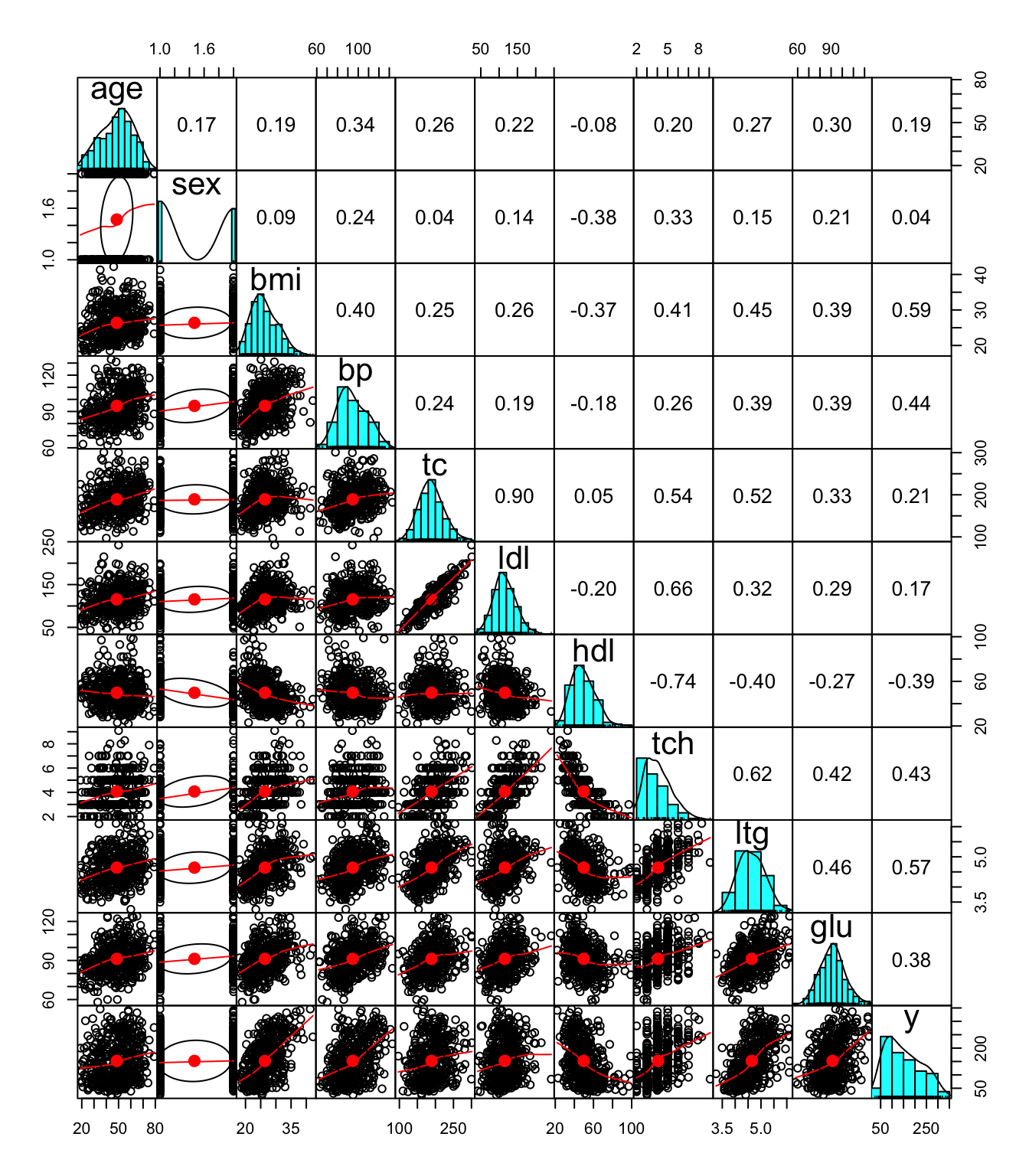
Some clear pattern is already apparent from the plot above: - The strong positive correlation between tc and ldl - The negative correlation between hdl and other variables including the response variable y
5.4 Four methods will be tried for prognostic modeling of the diabetes data
Full model: for this example, we have 442 records and 10 predictors, and we can afford to use the full model for prognostic modeling
The following three methods can be used to do variable selection, which is needed especially when the number of covariates is large. While it is not the case with this example, that is what we frequently encounter in biomarkers-related translational projects.
Lasso regression
Stepwise selection
Bayesian modeling with horseshoe priors
5.5 Full model for prognostic modeling
full_model_dia <- glm(glm(y ~ ., data=diabetes, family=gaussian(link="identity")))summary(full_model_dia)##
## Call:
## glm(formula = glm(y ~ ., data = diabetes, family = gaussian(link = "identity")))
##
## Deviance Residuals:
## Min 1Q Median 3Q Max
## -155.827 -38.536 -0.228 37.806 151.353
##
## Coefficients:
## Estimate Std. Error t value Pr(>|t|)
## (Intercept) -334.56714 67.45462 -4.960 1.02e-06 ***
## age -0.03636 0.21704 -0.168 0.867031
## sex -22.85965 5.83582 -3.917 0.000104 ***
## bmi 5.60296 0.71711 7.813 4.30e-14 ***
## bp 1.11681 0.22524 4.958 1.02e-06 ***
## tc -1.09000 0.57333 -1.901 0.057948 .
## ldl 0.74645 0.53083 1.406 0.160390
## hdl 0.37200 0.78246 0.475 0.634723
## tch 6.53383 5.95864 1.097 0.273459
## ltg 68.48312 15.66972 4.370 1.56e-05 ***
## glu 0.28012 0.27331 1.025 0.305990
## ---
## Signif. codes: 0 '***' 0.001 '**' 0.01 '*' 0.05 '.' 0.1 ' ' 1
##
## (Dispersion parameter for gaussian family taken to be 2932.682)
##
## Null deviance: 2621009 on 441 degrees of freedom
## Residual deviance: 1263986 on 431 degrees of freedom
## AIC: 4796
##
## Number of Fisher Scoring iterations: 25.5.1 Problems with the full model
Some of the clear pattern we saw in the full model are not evident in the full model results, because of the correlations between covariates. For example, we know that among all predictors, the single covariate that has a negative correlation with the outcome y is hdl from the previous correlation, but we cannot draw such conclusions from the full model results.
So it is not wise to just throw everything at the model and hope it will yield the correct results. We need to take into consideration the relationship between variables, let’s try the other three methods with covariate selection.
5.6 Lasso regression
From the lasso regression results below, we can see that 4 predictor variables of itg, hdl, bp and bmi are selected, with the hdl covariate being the one that has a negative coefficient. So this result agrees more with our previous correlation exploration than the full model result above.
library(glmnet)## Warning: package 'glmnet' was built under R version 4.1.2## Loading required package: Matrix## Warning: package 'Matrix' was built under R version 4.1.2## Loaded glmnet 4.1-4# glmnet requires x matrix (of predictors) and vector (values for y)
y = as.vector(diabetes$y)
x=as.matrix(diabetes[,-c(11)])
scaled.x=scale(x)
set.seed(123) # replicate results
lasso_model_dia <- cv.glmnet(scaled.x, y, alpha=1) # alpha = 1 lasso
best_lambda_dia <- lasso_model_dia$lambda.1se # largest lambda in 1 SE
lasso_coef <- lasso_model_dia$glmnet.fit$beta[, # retrieve coefficients
lasso_model_dia$glmnet.fit$lambda # at lambda.1se
== best_lambda_dia]
coef_la = data.table(lassoReg = lasso_coef) # build table
coef_la[, feature := names(lasso_coef)] # add feature names
to_plot_r_la = melt(coef_la # label table
, id.vars='feature'
, variable.name = 'model'
, value.name = 'coefficient')
ggplot(data=to_plot_r_la, # plot coefficients
aes(x=feature, y=coefficient, fill=model)) +
coord_flip() +
geom_bar(stat='identity', fill='brown4', color='blue') +
facet_wrap(~ model) + guides(fill=FALSE) ## Warning: `guides(<scale> = FALSE)` is deprecated. Please use `guides(<scale>
## = "none")` instead.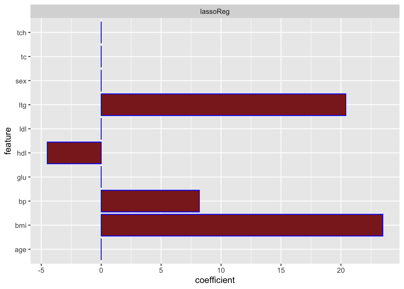
5.6.1 Examine the cross validation results of the lasso regression model and the best lambda values
plot(lasso_model_dia)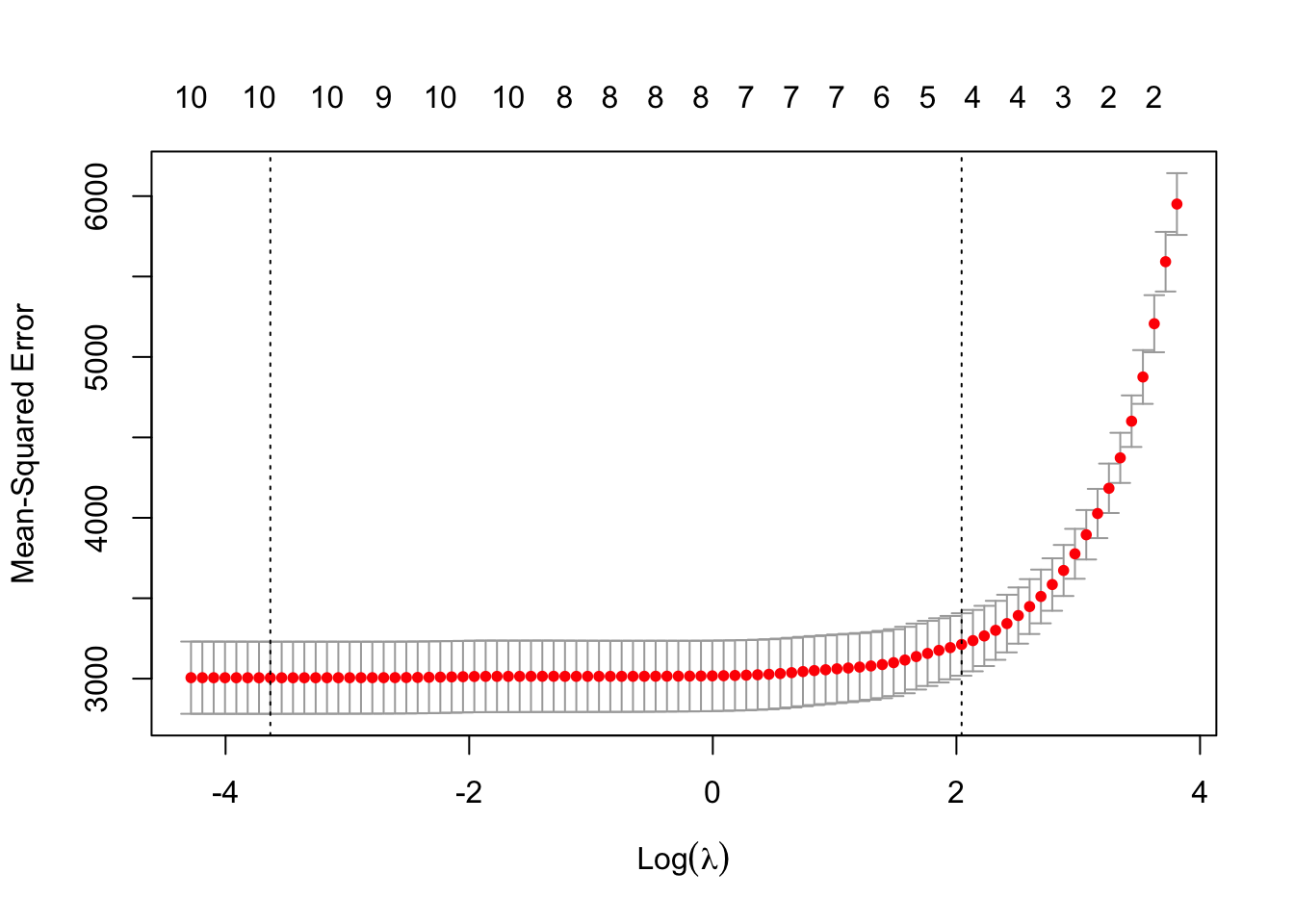
5.6.2 The lambda value 1 standard deviation away from the “optimal” lambda value by cross-validation, which can be used to fit the data to avoid overfitting
lasso_model_dia$lambda.1se## [1] 7.710415.6.3 The coefs plotted above
coef(lasso_model_dia, s = "lambda.1se")## 11 x 1 sparse Matrix of class "dgCMatrix"
## s1
## (Intercept) 152.133484
## age .
## sex .
## bmi 23.496545
## bp 8.190540
## tc .
## ldl .
## hdl -4.499227
## tch .
## ltg 20.407201
## glu .5.6.4 Refit a glm model using the lasso selected variables
sv_lasso_dia <- glm(glm(y ~ bmi + bp + hdl + ltg, data=diabetes, family=gaussian(link="identity")))
summary(sv_lasso_dia)
##
## Call:
## glm(formula = glm(y ~ bmi + bp + hdl + ltg, data = diabetes,
## family = gaussian(link = "identity")))
##
## Deviance Residuals:
## Min 1Q Median 3Q Max
## -142.104 -40.310 -3.297 39.139 151.831
##
## Coefficients:
## Estimate Std. Error t value Pr(>|t|)
## (Intercept) -263.2361 34.3467 -7.664 1.18e-13 ***
## bmi 5.9849 0.7095 8.435 4.87e-16 ***
## bp 0.9284 0.2148 4.323 1.91e-05 ***
## hdl -0.7141 0.2280 -3.132 0.00185 **
## ltg 44.2087 6.0787 7.273 1.64e-12 ***
## ---
## Signif. codes: 0 '***' 0.001 '**' 0.01 '*' 0.05 '.' 0.1 ' ' 1
##
## (Dispersion parameter for gaussian family taken to be 3049.857)
##
## Null deviance: 2621009 on 441 degrees of freedom
## Residual deviance: 1332787 on 437 degrees of freedom
## AIC: 4807.4
##
## Number of Fisher Scoring iterations: 25.7 Stepwise variable selection
Use both forward and backward feature selection
library(MASS)## Warning: package 'MASS' was built under R version 4.1.2##
## Attaching package: 'MASS'## The following object is masked from 'package:dplyr':
##
## selectbase_model <- lm(y~., data=diabetes)
results_stepwise_selection <- stepAIC(base_model,direction="both")## Start: AIC=3539.64
## y ~ age + sex + bmi + bp + tc + ldl + hdl + tch + ltg + glu
##
## Df Sum of Sq RSS AIC
## - age 1 82 1264068 3537.7
## - hdl 1 663 1264649 3537.9
## - glu 1 3080 1267066 3538.7
## - tch 1 3526 1267512 3538.9
## <none> 1263986 3539.6
## - ldl 1 5799 1269785 3539.7
## - tc 1 10600 1274586 3541.3
## - sex 1 44999 1308984 3553.1
## - ltg 1 56016 1320001 3556.8
## - bp 1 72100 1336086 3562.2
## - bmi 1 179033 1443019 3596.2
##
## Step: AIC=3537.67
## y ~ sex + bmi + bp + tc + ldl + hdl + tch + ltg + glu
##
## Df Sum of Sq RSS AIC
## - hdl 1 646 1264715 3535.9
## - glu 1 3001 1267069 3536.7
## - tch 1 3543 1267611 3536.9
## <none> 1264068 3537.7
## - ldl 1 5751 1269820 3537.7
## - tc 1 10569 1274637 3539.4
## + age 1 82 1263986 3539.6
## - sex 1 45830 1309898 3551.4
## - ltg 1 55964 1320032 3554.8
## - bp 1 73847 1337915 3560.8
## - bmi 1 179084 1443152 3594.2
##
## Step: AIC=3535.9
## y ~ sex + bmi + bp + tc + ldl + tch + ltg + glu
##
## Df Sum of Sq RSS AIC
## - glu 1 3093 1267808 3535.0
## - tch 1 3247 1267961 3535.0
## <none> 1264715 3535.9
## - ldl 1 7505 1272219 3536.5
## + hdl 1 646 1264068 3537.7
## + age 1 66 1264649 3537.9
## - tc 1 26839 1291554 3543.2
## - sex 1 46381 1311096 3549.8
## - bp 1 73533 1338248 3558.9
## - ltg 1 97508 1362223 3566.7
## - bmi 1 178542 1443256 3592.3
##
## Step: AIC=3534.98
## y ~ sex + bmi + bp + tc + ldl + tch + ltg
##
## Df Sum of Sq RSS AIC
## - tch 1 3686 1271494 3534.3
## <none> 1267808 3535.0
## - ldl 1 7472 1275280 3535.6
## + glu 1 3093 1264715 3535.9
## + hdl 1 738 1267069 3536.7
## + age 1 0 1267807 3537.0
## - tc 1 26378 1294186 3542.1
## - sex 1 44684 1312492 3548.3
## - bp 1 82152 1349960 3560.7
## - ltg 1 102520 1370328 3567.3
## - bmi 1 189976 1457784 3594.7
##
## Step: AIC=3534.26
## y ~ sex + bmi + bp + tc + ldl + ltg
##
## Df Sum of Sq RSS AIC
## <none> 1271494 3534.3
## + tch 1 3686 1267808 3535.0
## + glu 1 3533 1267961 3535.0
## + hdl 1 395 1271099 3536.1
## + age 1 11 1271483 3536.3
## - ldl 1 39377 1310871 3545.7
## - sex 1 41856 1313350 3546.6
## - tc 1 65236 1336730 3554.4
## - bp 1 79625 1351119 3559.1
## - bmi 1 190592 1462086 3594.0
## - ltg 1 294092 1565586 3624.2So the optimal variables selected by stepwise selection is sex + bmi + bp + tc + ldl + ltg
5.7.1 Refit a glm model using the stepwise selected variables
sv_step_dia <- glm(glm(y ~ sex + bmi + bp + tc + ldl + ltg, data=diabetes, family=gaussian(link="identity")))
summary(sv_step_dia)
##
## Call:
## glm(formula = glm(y ~ sex + bmi + bp + tc + ldl + ltg, data = diabetes,
## family = gaussian(link = "identity")))
##
## Deviance Residuals:
## Min 1Q Median 3Q Max
## -158.275 -39.476 -2.065 37.219 148.690
##
## Coefficients:
## Estimate Std. Error t value Pr(>|t|)
## (Intercept) -313.7666 25.3848 -12.360 < 2e-16 ***
## sex -21.5910 5.7056 -3.784 0.000176 ***
## bmi 5.7111 0.7073 8.075 6.69e-15 ***
## bp 1.1266 0.2158 5.219 2.79e-07 ***
## tc -1.0429 0.2208 -4.724 3.12e-06 ***
## ldl 0.8433 0.2298 3.670 0.000272 ***
## ltg 73.3065 7.3083 10.031 < 2e-16 ***
## ---
## Signif. codes: 0 '***' 0.001 '**' 0.01 '*' 0.05 '.' 0.1 ' ' 1
##
## (Dispersion parameter for gaussian family taken to be 2922.975)
##
## Null deviance: 2621009 on 441 degrees of freedom
## Residual deviance: 1271494 on 435 degrees of freedom
## AIC: 4790.6
##
## Number of Fisher Scoring iterations: 25.8 Bayesian modeling with horseshoe priors
We will use the brms package for the bayesian variable selection step
library(brms)## Warning: package 'brms' was built under R version 4.1.2## Loading required package: Rcpp## Warning: package 'Rcpp' was built under R version 4.1.2## Loading 'brms' package (version 2.17.0). Useful instructions
## can be found by typing help('brms'). A more detailed introduction
## to the package is available through vignette('brms_overview').##
## Attaching package: 'brms'## The following object is masked from 'package:psych':
##
## cs## The following object is masked from 'package:stats':
##
## arlibrary(tidyverse)## ── Attaching packages ─────────────────────────────────── tidyverse 1.3.1 ──## ✔ tibble 3.1.8 ✔ purrr 0.3.4
## ✔ tidyr 1.2.0 ✔ stringr 1.4.0
## ✔ readr 2.1.2 ✔ forcats 0.5.1## Warning: package 'tibble' was built under R version 4.1.2## Warning: package 'tidyr' was built under R version 4.1.2## Warning: package 'readr' was built under R version 4.1.2## ── Conflicts ────────────────────────────────────── tidyverse_conflicts() ──
## ✖ psych::%+%() masks ggplot2::%+%()
## ✖ psych::alpha() masks ggplot2::alpha()
## ✖ data.table::between() masks dplyr::between()
## ✖ tibble::column_to_rownames() masks textshape::column_to_rownames()
## ✖ textshape::combine() masks dplyr::combine()
## ✖ tidyr::expand() masks Matrix::expand()
## ✖ dplyr::filter() masks stats::filter()
## ✖ data.table::first() masks dplyr::first()
## ✖ purrr::flatten() masks textshape::flatten()
## ✖ dplyr::lag() masks stats::lag()
## ✖ data.table::last() masks dplyr::last()
## ✖ purrr::lift() masks caret::lift()
## ✖ tidyr::pack() masks Matrix::pack()
## ✖ MASS::select() masks dplyr::select()
## ✖ purrr::transpose() masks data.table::transpose()
## ✖ tidyr::unpack() masks Matrix::unpack()5.8.1 Variable selection horseshoe priors
We specify which variables as the base variables and which are subject to selection using the horseshoe prior. Because bmi and hdl have the best correlation (positive and negative) with the response variable y, we are going to use these two as the base variables, and the others as the ones subject to selection.
# For variable selection, scale the predictor and outcome to have unit variance
diabetes_std <- scale(diabetes)diabetes[1:2,]## age sex bmi bp tc ldl hdl tch ltg glu y
## 1 59 2 32.1 101 157 93.2 38 4 4.8598 87 151
## 2 48 1 21.6 87 183 103.2 70 3 3.8918 69 75n_cov = 10 # Number of variables
n_obs = nrow(diabetes) # Number of observations
n_p = 5 # prior info, number of optimal variables
#in horseshoe priors, another way to specify is the par_ratio (n_p/(n_cov - n_p))
p_tau = n_p/(n_cov - n_p) / sqrt(n_obs) # Shrinkage parameter tau,reference: Piironen et.al., 2016
fit_brms <- brm(
bf(y ~ x1 + x2,
formula("x1 ~ age + sex + bp + tc + ldl + tch + ltg + glu"),
formula("x2 ~ bmi + hdl"),
nl = TRUE),
data = diabetes_std, family = gaussian(),
prior = c(prior(horseshoe(df = 1, scale_global = p_tau, df_global = 1), class = "b",nlpar="x1"),
prior(normal(0, 1), class = "b",nlpar="x2")),
warmup = 1000, iter = 2000, chains = 4, cores = 4,
control = list(adapt_delta = 0.99, max_treedepth = 15),
seed = 1231)## Compiling Stan program...## Start sampling## Warning: There were 6 divergent transitions after warmup. See
## https://mc-stan.org/misc/warnings.html#divergent-transitions-after-warmup
## to find out why this is a problem and how to eliminate them.## Warning: Examine the pairs() plot to diagnose sampling problems5.8.2 Check the bayesian modeling results using horseshoe priors
summary(fit_brms)## Warning: There were 6 divergent transitions after warmup. Increasing
## adapt_delta above 0.99 may help. See http://mc-stan.org/misc/
## warnings.html#divergent-transitions-after-warmup## Family: gaussian
## Links: mu = identity; sigma = identity
## Formula: y ~ x1 + x2
## x1 ~ age + sex + bp + tc + ldl + tch + ltg + glu
## x2 ~ bmi + hdl
## Data: diabetes_std (Number of observations: 442)
## Draws: 4 chains, each with iter = 2000; warmup = 1000; thin = 1;
## total post-warmup draws = 4000
##
## Population-Level Effects:
## Estimate Est.Error l-95% CI u-95% CI Rhat Bulk_ESS Tail_ESS
## x2_Intercept -0.01 0.20 -0.51 0.40 1.00 1571 1177
## x2_bmi 0.34 0.04 0.25 0.42 1.00 5209 2875
## x2_hdl -0.15 0.06 -0.26 0.00 1.00 2258 1586
## x1_Intercept 0.01 0.20 -0.40 0.50 1.00 1515 1156
## x1_age -0.00 0.02 -0.06 0.05 1.00 4862 3445
## x1_sex -0.12 0.04 -0.20 -0.04 1.00 2846 1774
## x1_bp 0.18 0.04 0.10 0.26 1.00 4009 3080
## x1_tc -0.05 0.08 -0.25 0.05 1.00 1812 1824
## x1_ldl -0.01 0.06 -0.13 0.12 1.00 2360 2031
## x1_tch 0.01 0.06 -0.09 0.15 1.00 2736 2666
## x1_ltg 0.31 0.05 0.21 0.42 1.00 3672 3240
## x1_glu 0.02 0.03 -0.03 0.10 1.00 3650 3798
##
## Family Specific Parameters:
## Estimate Est.Error l-95% CI u-95% CI Rhat Bulk_ESS Tail_ESS
## sigma 0.71 0.02 0.66 0.75 1.00 5016 2826
##
## Draws were sampled using sampling(NUTS). For each parameter, Bulk_ESS
## and Tail_ESS are effective sample size measures, and Rhat is the potential
## scale reduction factor on split chains (at convergence, Rhat = 1).plot(fit_brms)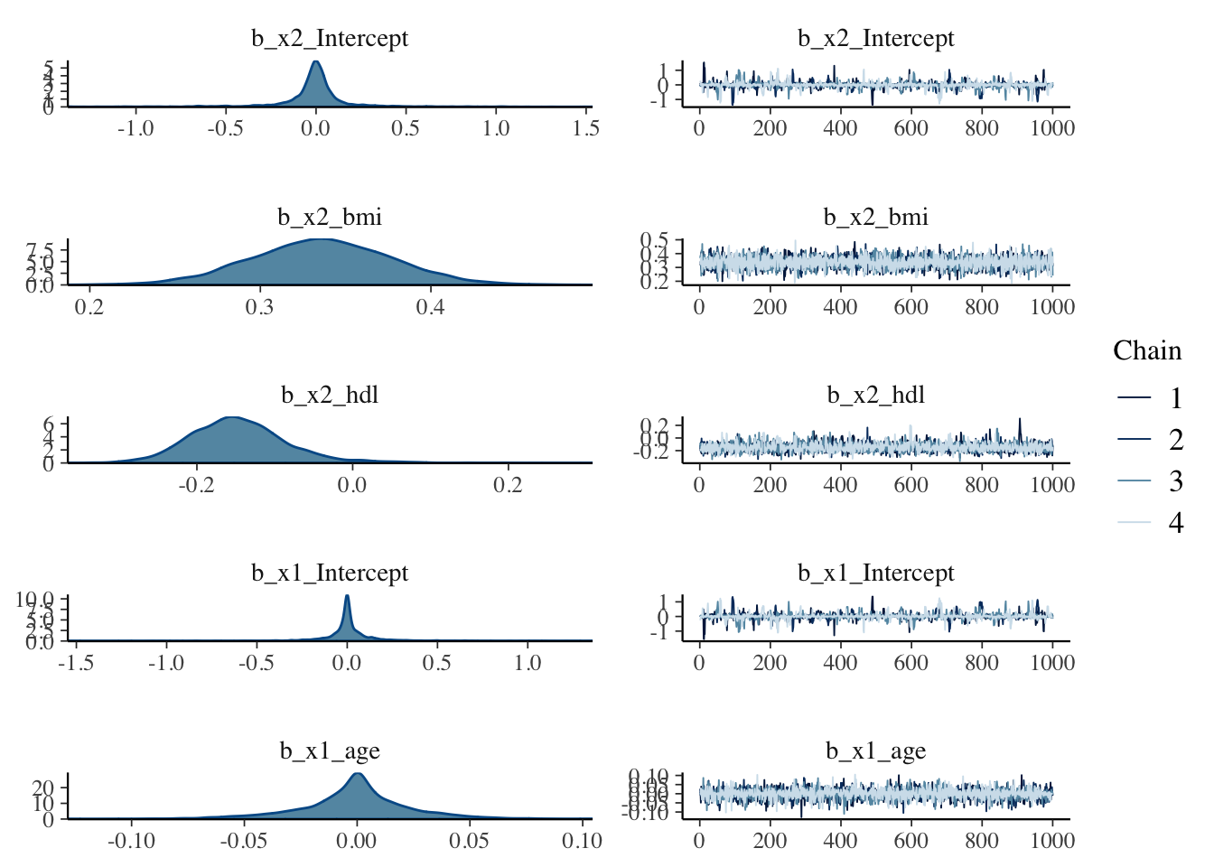
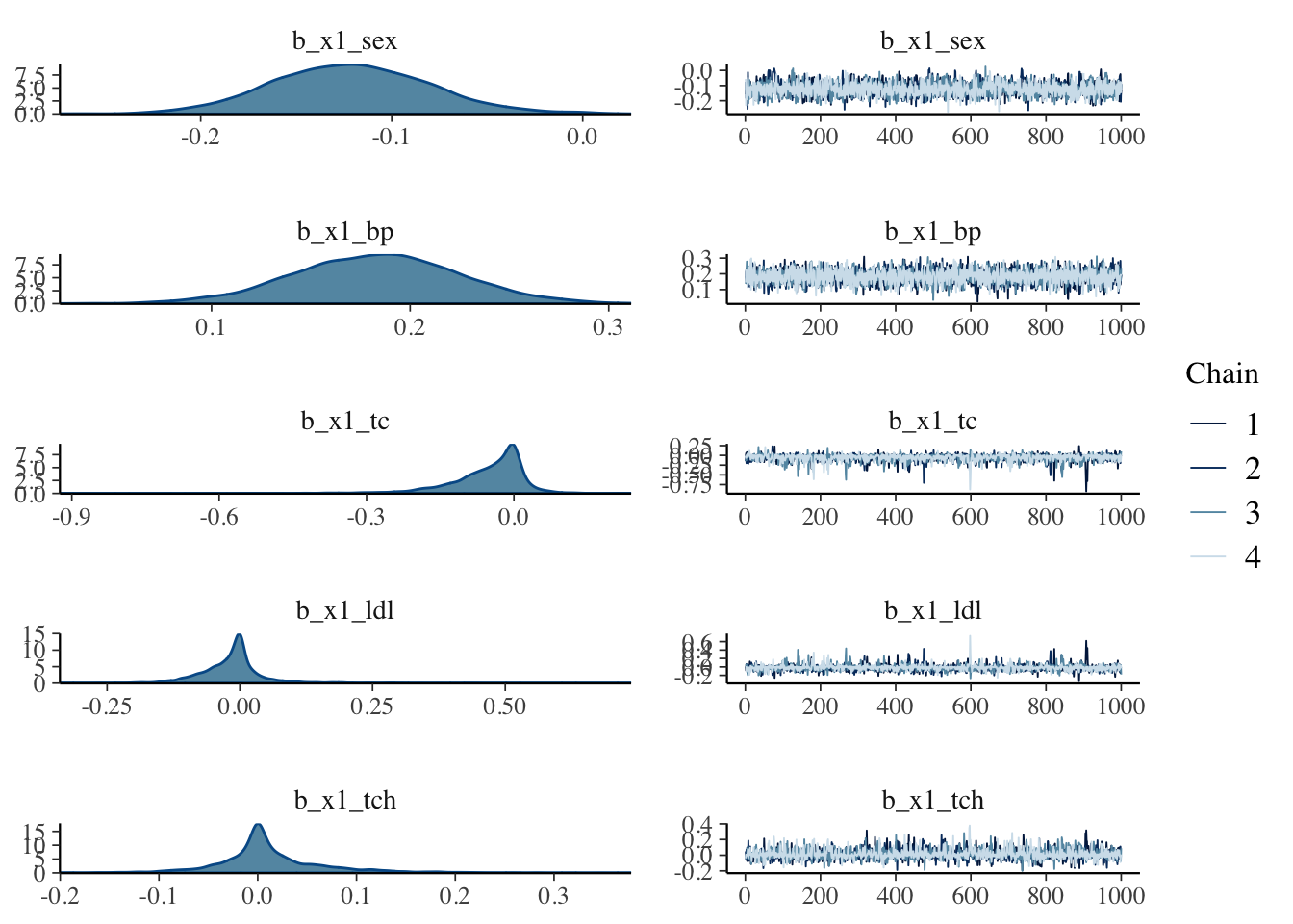
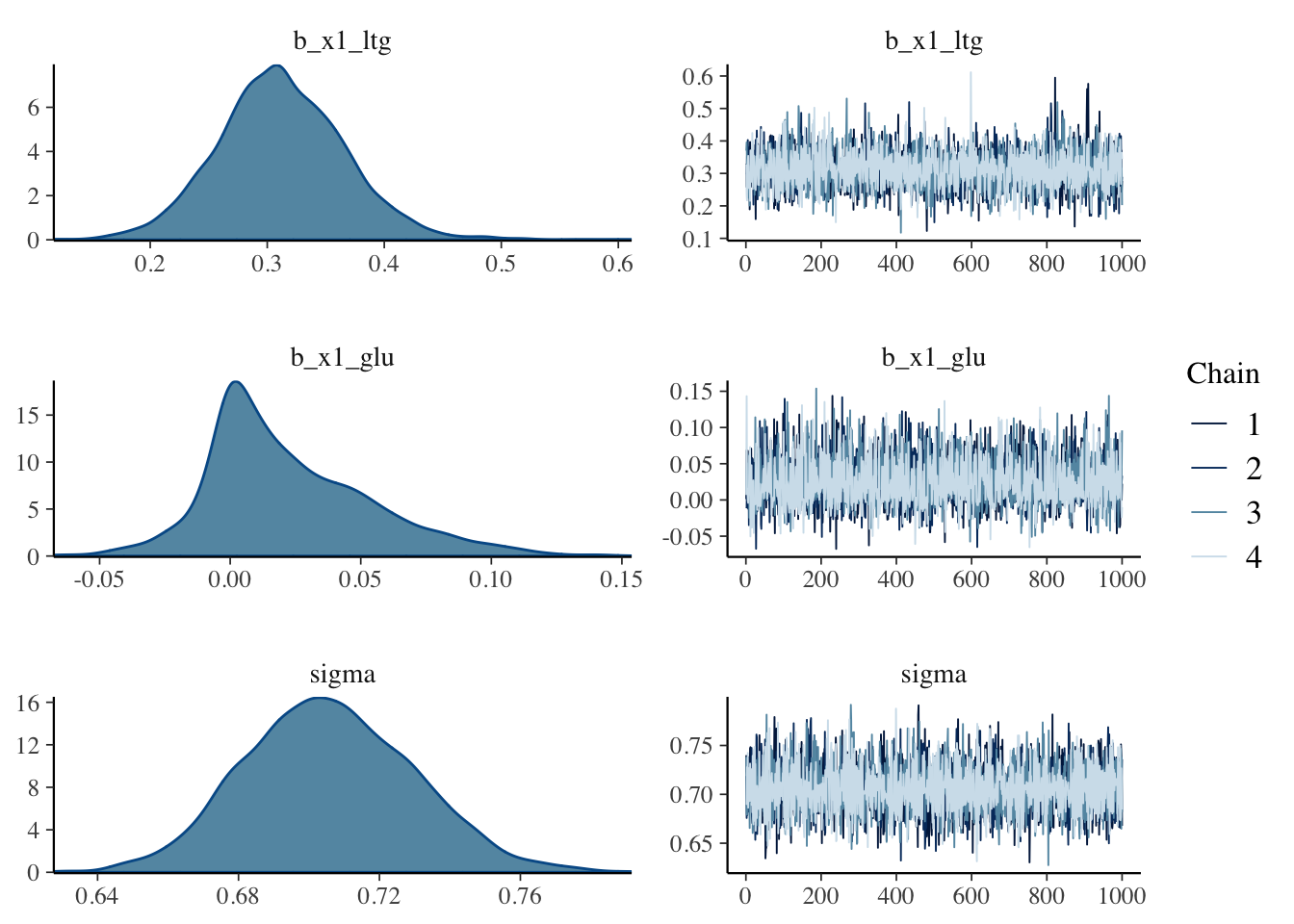
5.8.3 Check the posterier distribution of the horseshoe results
The data was scaled before modeling, so it has unit variance.
If the 95% confidence-interval of a variable is not overlapping with 0, we will consider it to be selected. So the plot below indicates that in addition to bmi and hdl (our base variables, which are not subject to horshoe prior selection), sex, bp and ltg are selected.
mcmc_plot(fit_brms)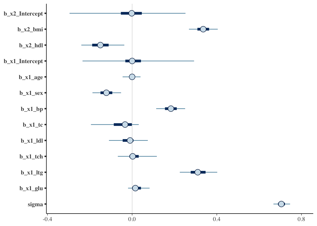
5.8.4 Refit a glm model using the horseshoe selected variables
sv_horseshoe_dia <- glm(glm(y ~ sex + bmi + bp + hdl + ltg, data=diabetes, family=gaussian(link="identity")))
summary(sv_horseshoe_dia)
##
## Call:
## glm(formula = glm(y ~ sex + bmi + bp + hdl + ltg, data = diabetes,
## family = gaussian(link = "identity")))
##
## Deviance Residuals:
## Min 1Q Median 3Q Max
## -150.031 -39.317 -0.561 37.307 148.382
##
## Coefficients:
## Estimate Std. Error t value Pr(>|t|)
## (Intercept) -217.6849 35.7638 -6.087 2.53e-09 ***
## sex -22.4742 5.7640 -3.899 0.000112 ***
## bmi 5.6431 0.7037 8.019 9.93e-15 ***
## bp 1.1232 0.2172 5.171 3.55e-07 ***
## hdl -1.0644 0.2417 -4.404 1.34e-05 ***
## ltg 43.2344 5.9874 7.221 2.32e-12 ***
## ---
## Signif. codes: 0 '***' 0.001 '**' 0.01 '*' 0.05 '.' 0.1 ' ' 1
##
## (Dispersion parameter for gaussian family taken to be 2953.856)
##
## Null deviance: 2621009 on 441 degrees of freedom
## Residual deviance: 1287881 on 436 degrees of freedom
## AIC: 4794.3
##
## Number of Fisher Scoring iterations: 25.9 Comparison of the models built using the different variable selection methods
One thing I would like to point out is that the numerical measure of model performance is one way of evaluating the results. It is not the only way, and it is not necessarily the best either.
We always need to have justifications from the scientific or clinical angles. Subject matter knowledge would be helpful. Why don’t we just rely the scientific or clinical inputs? Because they too have limitations. The fact we are using statistical models instead of physical models to perform the prognostic modeling suggests that we lack a good understanding of the science behind prognosis.
With the caveats and limitations states, let’s put the results together and compare them using BIC.
library(flexmix)## Warning: package 'flexmix' was built under R version 4.1.2BIC(full_model_dia)## [1] 4845.081BIC(sv_lasso_dia)## [1] 4831.961BIC(sv_step_dia)## [1] 4823.334BIC(sv_horseshoe_dia)## [1] 4822.903The 4 methods above yield decreasing BIC values. With BIC values, the lower the value, the better the goodness-of-fit. So our bayesian horseshoe prior approach appears to yield the better performance from this BIC numeric measure; at the same time, this approach also included our knowledge about the data by specifying the base variables (bmi and hdl). Based on the results, I would recommend using the bayesian horseshoe prior approach for variable selection to combine both great technical performance and the ability to incorportate subject matter knowledge.
5.10 More approaches are available for variable selection for prognostic modeling and other predictive modeling. For rexample, another bayesian-based variable selection method is called projection-based prediction, implemented in the R package “projpred”. There is a very good example vignettes available herer:
https://cran.r-project.org/web/packages/projpred/vignettes/projpred.html