Chapter 4 Dimensionality reduction
In data science, we are often faced with high dimensional data. In order to use high dimensional data in statistical or machine learning models, dimensionality reduction techniques need to be applied. We can reduce the dimensions of the data using methods like PCA or t-SNE to derive new features, or we can apply feature selection and extraction to filter the data. Along the way, differnt ways of visualizationare also going to be applied to demonstrate the applicabilities of the differnt methods and to explore and interpret the Pima Indian diabetes data.
The outline of the Dimensionality Reduction vignettes: (1) PCA and t-SNE (2) feature selection and feature extraction
4.1 setup the environment
library(dplyr)##
## Attaching package: 'dplyr'## The following objects are masked from 'package:stats':
##
## filter, lag## The following objects are masked from 'package:base':
##
## intersect, setdiff, setequal, unionlibrary(caret)## Warning: package 'caret' was built under R version 4.1.2## Loading required package: ggplot2## Warning: package 'ggplot2' was built under R version 4.1.2## Loading required package: latticelibrary(Rtsne)## Warning: package 'Rtsne' was built under R version 4.1.2library(ggplot2)
library(psych)## Warning: package 'psych' was built under R version 4.1.2##
## Attaching package: 'psych'## The following objects are masked from 'package:ggplot2':
##
## %+%, alphalibrary(ggfortify)## Warning: package 'ggfortify' was built under R version 4.1.2library(textshape)##
## Attaching package: 'textshape'## The following object is masked from 'package:dplyr':
##
## combinelibrary(mlbench)4.2 load and explore the data
4.2.1 load the data
data("PimaIndiansDiabetes")
str(PimaIndiansDiabetes)
## 'data.frame': 768 obs. of 9 variables:
## $ pregnant: num 6 1 8 1 0 5 3 10 2 8 ...
## $ glucose : num 148 85 183 89 137 116 78 115 197 125 ...
## $ pressure: num 72 66 64 66 40 74 50 0 70 96 ...
## $ triceps : num 35 29 0 23 35 0 32 0 45 0 ...
## $ insulin : num 0 0 0 94 168 0 88 0 543 0 ...
## $ mass : num 33.6 26.6 23.3 28.1 43.1 25.6 31 35.3 30.5 0 ...
## $ pedigree: num 0.627 0.351 0.672 0.167 2.288 ...
## $ age : num 50 31 32 21 33 30 26 29 53 54 ...
## $ diabetes: Factor w/ 2 levels "neg","pos": 2 1 2 1 2 1 2 1 2 2 ...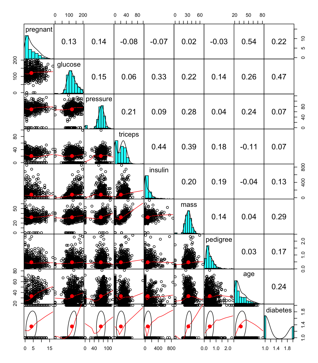
4.3 Dimensionality reduction methods: PCA
4.3.1 Run PCA and print out the summary
You can see that that the 1st components captures 26.2% of the variance in the data, 2nd component captures 21.6% of the variance in the data … For this dataset, the first two components together only help to explain only 47.8% of the variance in the data.
prin_components <- prcomp(PimaIndiansDiabetes[-c(9)],
             center = TRUE,
            scale. = TRUE)
summary(prin_components)
## Importance of components:
## PC1 PC2 PC3 PC4 PC5 PC6 PC7
## Standard deviation 1.4472 1.3158 1.0147 0.9357 0.87312 0.82621 0.64793
## Proportion of Variance 0.2618 0.2164 0.1287 0.1094 0.09529 0.08533 0.05248
## Cumulative Proportion 0.2618 0.4782 0.6069 0.7163 0.81164 0.89697 0.94944
## PC8
## Standard deviation 0.63597
## Proportion of Variance 0.05056
## Cumulative Proportion 1.00000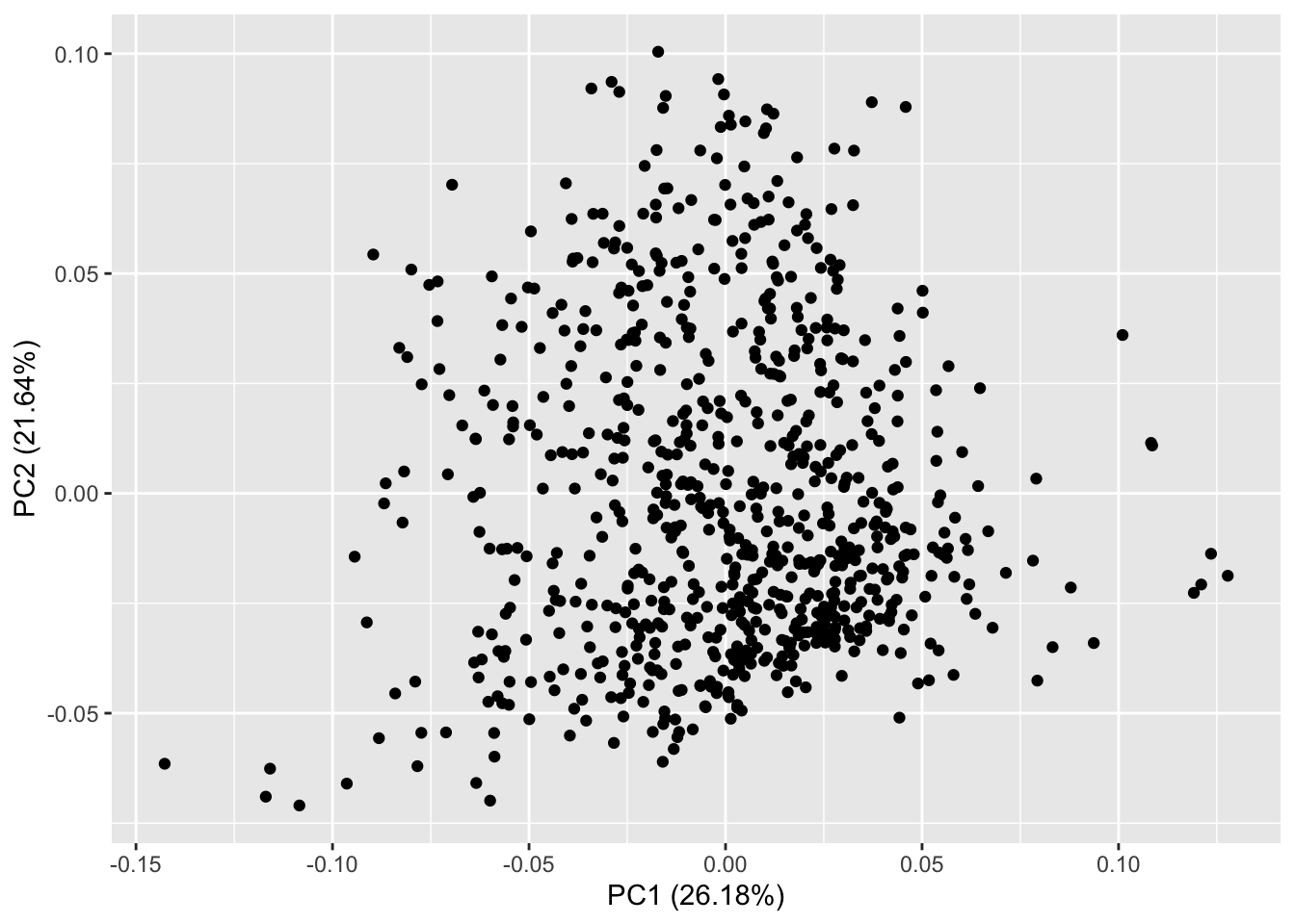 ### You can visualize glucose and diabetes together in the PCA plot
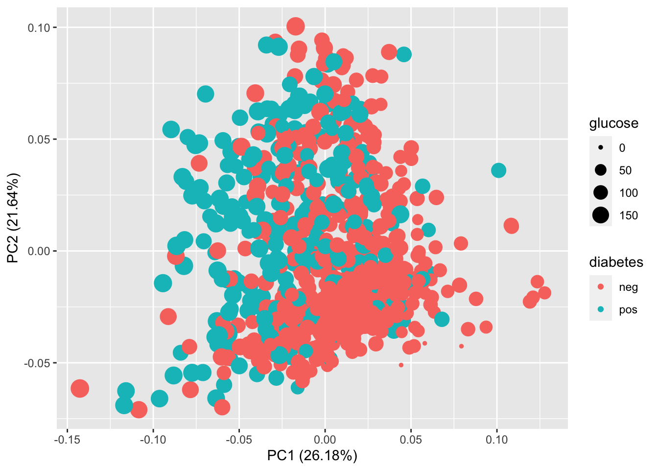
4.4 Dimensionality method: t-SNE
4.4.1 run t-SNE and extract the t-SNE components
set.seed(1342)
for_tsne <- PimaIndiansDiabetes %>%
  dplyr::mutate(PatientID=dplyr::row_number())
tsne_trans <- for_tsne %>%
  dplyr::select(where(is.numeric)) %>%
  column_to_rownames("PatientID") %>%
  scale() %>%
  Rtsne()

tsne_df <- tsne_trans$Y %>%
  as.data.frame() %>%
  dplyr::rename(tsne1="V1",
         tsne2="V2") %>%
  dplyr::mutate(PatientID=dplyr::row_number()) %>%
  dplyr::inner_join(for_tsne, by="PatientID")
4.4.2 plot the t-SNE results: a non-linear representation of the data; you can clearly see a better separation of diabetes neg and pos patients, although still not good enough.
ggplot(tsne_df,aes(x = tsne1,
             y = tsne2,
             size=glucose,
             color = diabetes))+
  geom_point(alpha=0.4)+
  theme(legend.position="right")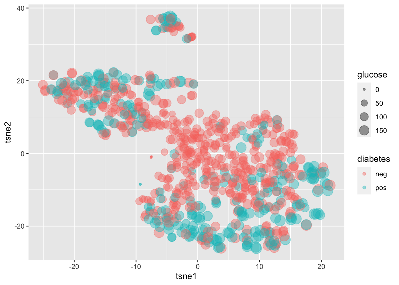
4.5 Feature selection and extraction for machine learning modeling
There are roughly two groups of feature selection methods: wrapper methods and filter methods.
Wrapper methods evaluate subsets of variables which allows to detect the possible interactions amongst variables.The two main disadvantages of these methods are: (1) The increasing overfitting risk when the number of observations is insufficient. (2) The significant computation time when the number of variables is large
Filter type methods select variables regardless of the model. They are based only on general features like the correlation with the variable to predict. Filter methods suppress the least interesting variables. The other variables will be part of a classification or a regression model used to classify or to predict data. These methods are particularly effective in computation time and robust to overfitting.
Below are a couple of examples:
4.5.1 wrapper method: recursive feature elimination (rfe)
Preliminary conclusions: The top 5 variables (out of 6): pedigree, pregnant, mass, glucose, age
One technical detail: the rfe function does not work when the outcome “y” is factor (which is the case for the dataset), which needs to be converted into numeric.
set.seed(1342)
feature_size_list <-  c(1:8) # for a total of 8 predictors

rfe_ctrl <- rfeControl(functions = lmFuncs,
                   method = "repeatedcv",
                   repeats = 5,
                   verbose = FALSE)

rfe_results <- rfe(PimaIndiansDiabetes[,-which(colnames(PimaIndiansDiabetes) %in% c("diabetes"))], as.numeric(PimaIndiansDiabetes$diabetes),
                 sizes = feature_size_list,
                 rfeControl = rfe_ctrl)

rfe_results
##
## Recursive feature selection
##
## Outer resampling method: Cross-Validated (10 fold, repeated 5 times)
##
## Resampling performance over subset size:
##
## Variables RMSE Rsquared MAE RMSESD RsquaredSD MAESD Selected
## 1 0.4702 0.04176 0.4417 0.01884 0.03902 0.01626
## 2 0.4578 0.08930 0.4184 0.02121 0.05336 0.01906
## 3 0.4404 0.15662 0.3919 0.02354 0.06471 0.02230
## 4 0.4032 0.29231 0.3383 0.02730 0.08237 0.02310
## 5 0.4051 0.28577 0.3392 0.02722 0.08111 0.02349
## 6 0.4024 0.29418 0.3363 0.02599 0.07862 0.02246 *
## 7 0.4034 0.29058 0.3370 0.02596 0.07800 0.02258
## 8 0.4037 0.28923 0.3373 0.02566 0.07637 0.02260
##
## The top 5 variables (out of 6):
## pedigree, pregnant, mass, glucose, age4.5.2 filter method: single variate filtering method where the features are pre-screened using simple univariate statistical methods, and then only those that pass the criteria are selected for subsequent modeling.
Preliminary conclusions from the results: On average, the top 5 selected variables (out of a possible 8): age (100%), glucose (100%), insulin (100%), mass (100%), pedigree (100%)
set.seed(1342)
filter_Ctrl <- sbfControl(functions = rfSBF, method = "repeatedcv", repeats = 5)
filter_results <- sbf(PimaIndiansDiabetes[,-which(colnames(PimaIndiansDiabetes) %in% c("diabetes"))], PimaIndiansDiabetes$diabetes, sbfControl = filter_Ctrl)
filter_results
##
## Selection By Filter
##
## Outer resampling method: Cross-Validated (10 fold, repeated 5 times)
##
## Resampling performance:
##
## Accuracy Kappa AccuracySD KappaSD
## 0.7557 0.4464 0.04189 0.09284
##
## Using the training set, 7 variables were selected:
## pregnant, glucose, triceps, insulin, mass...
##
## During resampling, the top 5 selected variables (out of a possible 8):
## age (100%), glucose (100%), insulin (100%), mass (100%), pedigree (100%)
##
## On average, 6.7 variables were selected (min = 6, max = 8)