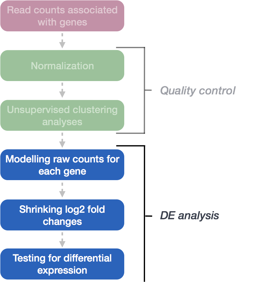
Chapter 5 Negative Binomial model fitting
5.1 Generalized Linear Model fit for each gene
The final step in the DESeq2 workflow is fitting the Negative Binomial model for each gene and performing differential expression testing.
Exercise points = +1
In the DESeq2 workflow, what is the purpose of the design matrix in the context of fitting the Negative Binomial model for each gene?
DESeq2 fits the Negative Binomial model to the normalized count data for each gene, taking into account the size factors and dispersion estimates calculated earlier. The model estimates beta coefficients for each experimental condition – these are the statistical parameters that represent the log2 fold changes for each experimental condition compared to the baseline. For example, if your experiment compares MOV10 overexpression vs. control, DESeq2 calculates a beta coefficient that tells you how much gene expression changed due to the MOV10 overexpression (on the log2 scale).
However, these initial log2 fold change estimates can be unreliable for genes with low counts or high dispersion. These genes have high uncertainty in their fold change estimates (large lfcSE), which can lead to inflated fold changes that may not be biologically meaningful.
5.2 Shrunken log2 foldchanges (LFC)
To generate more accurate log2 foldchange estimates, DESeq2 allows for the shrinkage of the LFC estimates toward zero when the information for a gene is low, which could include:
- Low counts
- High dispersion values
As with the shrinkage of dispersion estimates, LFC shrinkage uses information from all genes to generate more accurate estimates. DESeq2 looks at the pattern of fold changes across all genes in your dataset and uses this information to adjust estimates for genes with little reliable data (low counts or high dispersion) toward more reasonable values.
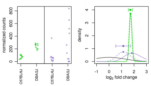
For example, in the figure above, Looking at the figure, the green and purple genes both show similar average expression levels between the two sample groups, but they differ in how much variability they have. The green gene has very consistent values (low variability), while the purple gene has much more scattered data points (high variability). Because the green gene has reliable, consistent data, DESeq2 doesn’t need to adjust its fold change estimate much - the original and adjusted estimates are nearly the same. However, for the purple gene with noisy, variable data, DESeq2 pulls the fold change estimate toward a more moderate value to account for the uncertainty.
This shows how DESeq2 tailors the amount of adjustment based on data quality - reliable genes get little adjustment, while noisy genes get more adjustment toward reasonable values.
To generate the shrunken log2 fold change estimates, you have to run an additional step on your results object (that we will create below) with the function lfcShrink().
NOTE: LFC shrinkage does not change which genes are called significantly differentially expressed (determined by padj values). It only provides more accurate fold change estimates for downstream analysis. Shrunk LFCs are particularly important for: - Ranking genes by effect size - Subsetting significant genes by fold change thresholds
- Functional analysis tools like GSEA that use fold changes as input - Visualization and interpretation of results
5.3 Hypothesis testing using the Wald test
For each gene, DESeq2 tests whether there is a significant difference in expression between your experimental conditions.
Null hypothesis (H₀): There is no difference between groups (log2 fold change = 0)
DESeq2 uses the Wald test to calculate a p-value for each gene, which represents the probability of observing a fold change this large (or larger) if the null hypothesis were true. If the p-value is small (typically < 0.05 after multiple testing correction), we reject the null hypothesis and conclude the gene is differentially expressed.
5.4 Creating contrasts
To indicate to DESeq2 the two groups we want to compare, we can use contrasts. A contrast is provided to DESeq2 as an argument in the results() function, the function that performs differential expression testing using the Wald test.
In the contrast you can specify the comparison of interest and the levels to compare. The level given last is the base level for the comparison. The syntax is given below:
# General syntax
contrast <- c("condition", "level_to_compare", "base_level")
results(dds, contrast = contrast)
5.4.0.1 MOV10 DE analysis: contrasts and Wald tests
We have three sample classes so we can make three possible pairwise comparisons:
- Control vs. Mov10 overexpression
- Control vs. Mov10 knockdown
- Mov10 knockdown vs. Mov10 overexpression
We are really only interested in #1 and #2 from above. Using the design formula we provided ~ sampletype, indicating that this is our main factor of interest.
5.4.1 Building the results table
To build our results table we will use the results() function. To specify which groups to compare, we supply the contrast using the contrast argument. In this example, we’ll first extract the unshrunken results for MOV10 overexpression vs. Control, then apply log2 fold change shrinkage.
# Define contrasts
contrast_oe <- c("sampletype",
                 "MOV10_overexpression",
                 "control")

# Extract results table (unshrunken)
res_tableOE_unshrunken <- results(dds, contrast = contrast_oe)

# Check available coefficients for shrinkage
resultsNames(dds)
## [1] "Intercept"
## [2] "sampletype_MOV10_knockdown_vs_control"
## [3] "sampletype_MOV10_overexpression_vs_control"# Shrink log2 fold changes
res_tableOE <- lfcShrink(dds = dds,
coef = "sampletype_MOV10_overexpression_vs_control",
res = res_tableOE_unshrunken)
# Save the results for future use
saveRDS(res_tableOE, file = "data/res_tableOE.RDS")Understanding the contrast order:
This calculates fold changes as: MOV10_overexpression / control
Interpreting the results:
Positive log2FC → gene is upregulated in MOV10_overexpression (higher expression than control)
Negative log2FC → gene is downregulated in MOV10_overexpression (lower expression than control)
For example, log2FC = -2 means the gene has 4-fold lower expression in MOV10_overexpression compared to control.
STOPPED HERE
5.4.2 MA Plot
The MA plot shows the relationship between expression level (mean of normalized counts) and log2 fold change for all genes. This is useful for: - Visualizing the effect of LFC shrinkage - Identifying the distribution of DE genes across expression levels - Quality checking your results
Significantly DE genes are colored for easy identification.
Unshrunken results:
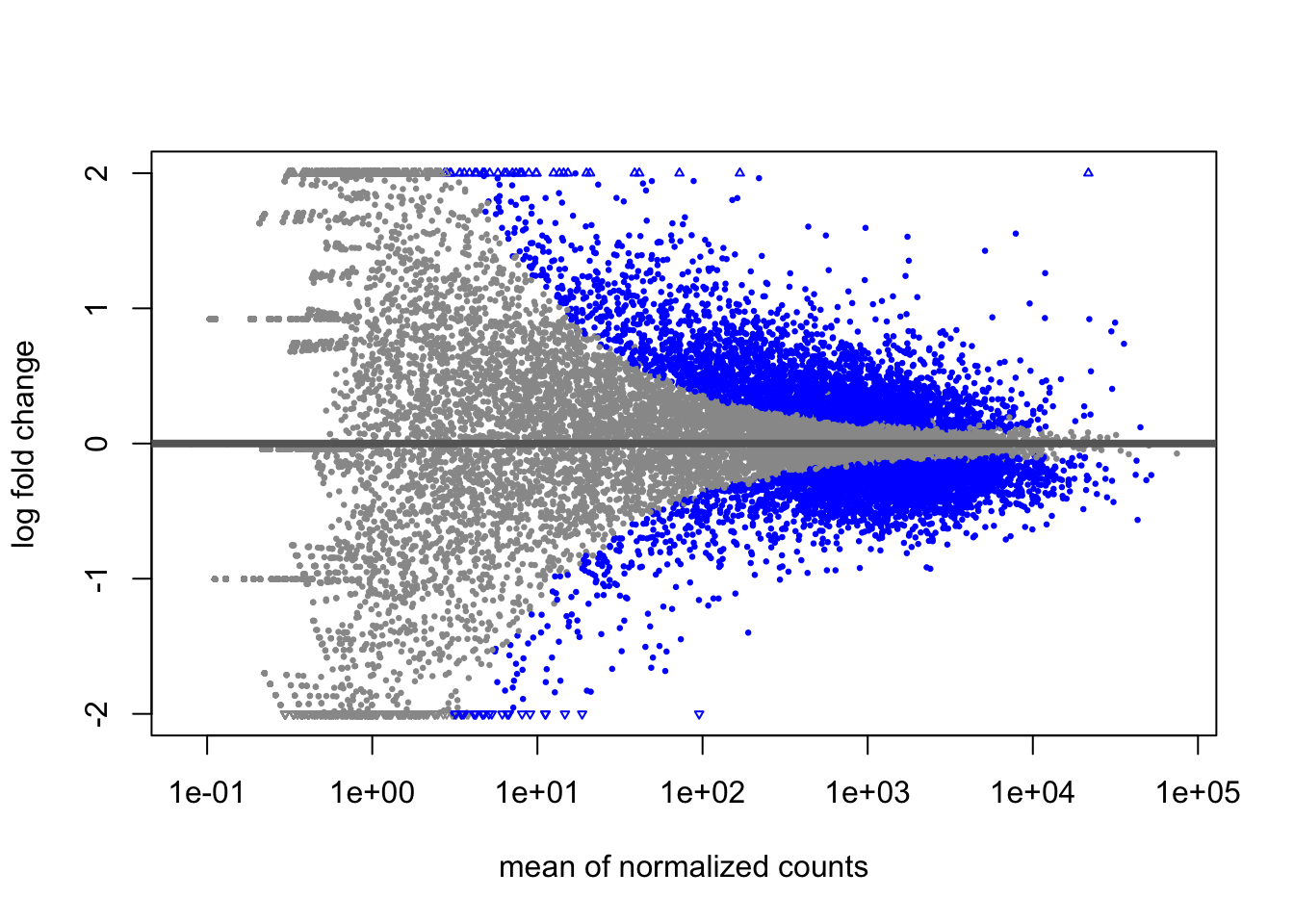
Notice the wide spread of fold changes, especially for low-expression genes.
Shrunken results:
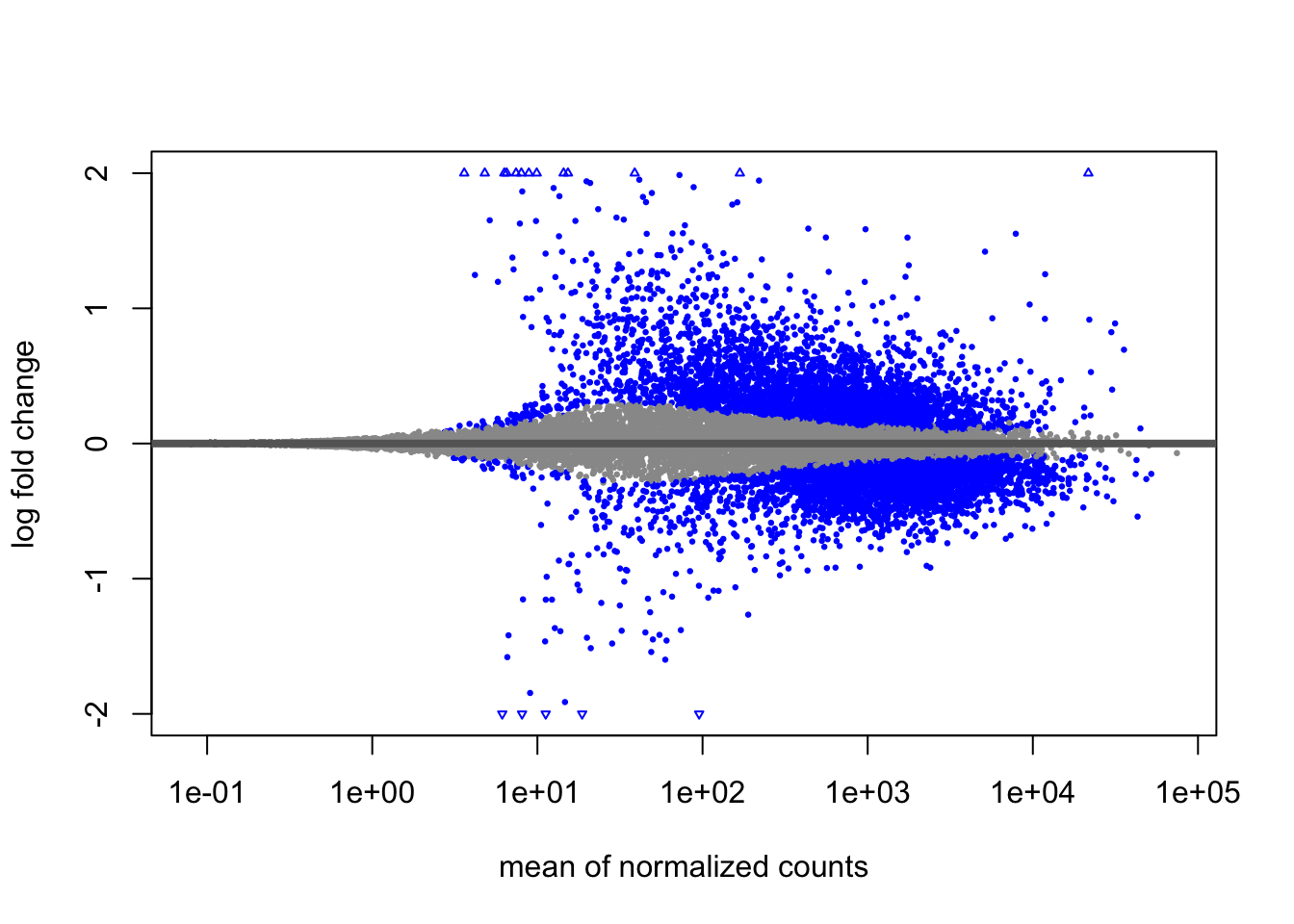
After shrinkage, extreme fold changes from low-count genes are moderated, while high-confidence changes are preserved.
What to look for: Significant genes should be distributed across expression levels. If all your DE genes are low-expression, this may indicate quality issues.
5.4.3 MOV10 DE analysis: results exploration
The results table looks very much like a data.frame and in many ways it can be treated like one (i.e when accessing/subsetting data). However, it is important to recognize that it is actually stored in a DESeqResults object. When we start visualizing our data, this information will be helpful.
## [1] "DESeqResults"
## attr(,"package")
## [1] "DESeq2"
Let’s go through some of the columns in the results table to get a better idea of what we are looking at. To extract information regarding the meaning of each column we can use mcols():
## DataFrame with 5 rows and 2 columns
##                        type            description
##                 <character>            <character>
## baseMean       intermediate mean of normalized c..
## log2FoldChange      results log2 fold change (MA..
## lfcSE               results posterior SD: sample..
## pvalue              results Wald test p-value: s..
## padj results BH adjusted p-values- baseMean: intermediate mean of normalized counts for all samples
- log2FoldChange: results log2 fold change (MLE): condition MOV10_overexpression vs control
- lfcSE: results standard error: condition MOV10_overexpression vs control
- pvalue: results Wald test p-value: condition MOV10_overexpression vs control
- padj: results BH adjusted p-values
5.5 Understanding lfcSE (Standard Error)
The lfcSE tells you how confident you should be in the log2 fold change estimate.
\[\text{lfcSE} = \sqrt{\text{Var}(\log_2 FC)}\]
In plain English: lfcSE measures how much your fold change estimate might vary if you repeated the experiment.
5.5.1 What makes lfcSE large (= less confident)?
- Low expression genes - Few reads means noisy estimates
- High variability between replicates - Inconsistent measurements
- Few replicates - Less data to estimate from
5.5.2 What makes lfcSE small (= more confident)?
- High expression genes - Many reads means precise estimates
- Consistent replicates - Reliable measurements
- More replicates - More data to work with
5.5.3 Example:
Gene A:
log2FC = 2.5
lfcSE = 0.2 ← Small error, confident estimate
Gene B:
log2FC = 2.5
lfcSE = 1.8 ← Large error, uncertain estimate
Both genes show the same fold change, but we trust Gene A’s estimate much more.
5.5.4 Why does this matter?
DESeq2 uses the Wald test to ask: “Is the fold change big compared to the uncertainty?”
\[\text{Wald statistic} = \frac{\text{log2FC}}{\text{lfcSE}}\]
- Gene A: \(2.5 / 0.2 = 12.5\) → Large statistic → Small p-value → Significant
- Gene B: \(2.5 / 1.8 = 1.4\) → Small statistic → Large p-value → Not significant
Key insight: A big fold change with high uncertainty may not be significant, while a smaller fold change with low uncertainty can be highly significant.
5.5.5 From Wald statistic to p-value
Once we calculate the Wald statistic: \[W = \frac{\text{log2FC}}{\text{lfcSE}}\]
DESeq2 converts it to a p-value using the standard normal distribution.
The logic:
If the null hypothesis is true (no real fold change), the Wald statistic should be close to 0
Large |W| values are unlikely under the null hypothesis
The p-value tells us: “How unlikely is a value this extreme?”
Hypothesis testing using the Wald test
The first step in hypothesis testing is to set up a null hypothesis for each gene. In our case, the null hypothesis is that there is no differential expression across the two sample groups (LFC == 0). Notice that we can do this without observing any data, because it is based on a thought experiment. Second, we use a statistical test to determine if based on the observed data, the null hypothesis is true.
With DESeq2, the Wald test is commonly used for hypothesis testing when comparing two groups. A Wald test statistic is computed along with a probability that a test statistic at least as extreme as the observed value were selected at random. This probability is called the p-value of the test. If the p-value is small we reject the null hypothesis and state that there is evidence against the null (i.e. the gene is differentially expressed).
Now let’s take a look at what information is stored in the results:
## log2 fold change (MAP): sampletype MOV10_overexpression vs control
## Wald test p-value: sampletype MOV10 overexpression vs control
## DataFrame with 6 rows and 5 columns
##               baseMean log2FoldChange     lfcSE    pvalue      padj
##              <numeric>      <numeric> <numeric> <numeric> <numeric>
## 1/2-SBSRNA4  45.652040     0.16820235  0.209100 0.1610752 0.2750250
## A1BG         61.093102     0.13645896  0.176779 0.2401909 0.3716156
## A1BG-AS1    175.665807    -0.04046122  0.116928 0.6789312 0.7840468
## A1CF          0.237692     0.00626747  0.210057 0.7945932        NA
## A2LD1        89.617985     0.29017719  0.195395 0.0333343 0.0774672
## A2M 5.860084 -0.09619722 0.233561 0.1057823 0.1976308## [1] "baseMean" "log2FoldChange" "lfcSE" "pvalue"
## [5] "padj"In some cases, p-values or adjusted p-values may be set to NA for a gene. This happens in three scenarios:
Zero counts: If all samples have zero counts for a gene, its baseMean will be zero, and the log2 fold change, p-value, and adjusted p-value will all be set to NA.
Outliers: If a gene has an extreme count outlier, its p-values will be set to NA. These outliers are detected using Cook’s distance.
Cook’s Distance
What it measures: How much one sample is “pulling” the results for a gene.
Why we care: - Outlier samples can make genes appear significant when they’re not - Or hide real differences
What DESeq2 does:
- Calculates Cook’s distance for every sample and gene
- If any sample has unusually high influence, sets the gene’s p-value to NA
- This is a quality control measure to prevent false positives
- Low counts: If a gene is filtered out by independent filtering for having a low mean normalized count, only the adjusted p-value will be set to NA.
5.5.6 Multiple test correction
Note that we have pvalues and p-adjusted values in the output. Which should we use to identify significantly differentially expressed genes?
If we used the p-value directly from the Wald test with a significance cut-off of p < 0.05, that means there is a 5% chance that any single significant result is a false positive. Each p-value is the result of a single test (single gene). The more genes we test, the more we inflate the overall false positive rate.
This is the multiple testing problem. For example, if we test 20,000 genes for differential expression, at p < 0.05 we would expect to find 1,000 genes by chance. If we found 3000 genes to be differentially expressed total, roughly one third of our genes are false positives. We would not want to sift through our “significant” genes to identify which ones are true positives.
DESeq2 helps reduce the number of genes tested by removing those genes unlikely to be significantly DE prior to testing, such as those with low number of counts and outlier samples (gene-level QC). However, we still need to correct for multiple testing to reduce the number of false positives.
FDR/Benjamini-Hochberg: The Benjamini-Hochberg (BH) method controls the False Discovery Rate - the expected proportion of false positives among your significant results.
How it works: 1. Rank all genes by p-value (smallest to largest) 2. Adjust each p-value:
\[\text{padj} = p \times \frac{m}{\text{rank}}\]
Where:
- m = total number of genes tested
- rank = position in the sorted list (1 for smallest p-value)
Example of BH adjustment:
Testing 20,000 genes:
Gene A: p = 0.00001, rank = 1 → padj = 0.00001 × (20000/1) = 0.2
Gene B: p = 0.0001, rank = 50 → padj = 0.0001 × (20000/50) = 0.04
Gene C: p = 0.001, rank = 500 → padj = 0.001 × (20000/500) = 0.04
Notice how the adjustment gets smaller for genes with better ranks!
The intuition: Genes with very small p-values (high ranks) get smaller adjustments, while genes with moderate p-values get larger penalties because you’re testing so many genes.
DESeq2 implements this automatically - you just need to use padj instead of pvalue.
In DESeq2, the p-values attained by the Wald test are corrected for multiple testing using the Benjamini and Hochberg method by default. There are options to use other methods in the results() function. The p-adjusted values should be used to determine significant genes. The significant genes can be output for visualization and/or functional analysis.
So what does FDR < 0.05 mean? By setting the FDR cutoff to < 0.05, we’re saying that the proportion of false positives we expect amongst our differentially expressed genes is 5%. For example, if you call 500 genes as differentially expressed with an FDR cutoff of 0.05, you expect 25 of them to be false positives.
Example: Suppose we test 20,000 genes for differential expression.
| Threshold | Genes called significant | Expected false positives |
|---|---|---|
| p < 0.05 (unadjusted) | 3000 | ~1000 (33%) |
| padj < 0.05 (BH adjusted) | 500 | ~25 (5%) |
Unadjusted: 20,000 genes × 0.05 = 1,000 false positives expected just by chance!
BH adjusted: 500 significant genes × 0.05 = 25 false positives expected - much better!
Now, we can filter the table to retain only the genes that meet the significance and fold change criteria.
5.5.7 Extracting Significant Differentially Expressed Genes
In some cases, using only the FDR threshold doesn’t sufficiently reduce the number of significant genes, making it difficult to extract biologically meaningful results. To increase stringency, we can apply an additional fold change threshold.
Let’s start by setting the thresholds for both adjusted p-value (FDR < 0.05) and log2 fold change (|log2FC| > 0.58, corresponding to a 1.5-fold change):
Next, we’ll convert the results table to a tibble for easier subsetting:
Now, we can filter the table to retain only the genes that meet the significance and fold change criteria:
sigOE <- res_tableOE_tb %>%
  dplyr::filter(padj < padj.cutoff &
                abs(log2FoldChange) > lfc.cutoff)

# Save the results for future use
saveRDS(sigOE,"data/sigOE.RDS")
Exercise points = +2
How many genes are differentially expressed in the Overexpression vs. Control comparison based on the criteria we just defined?
Does this reduce our results? How many genes are differentially expressed in the Overexpression vs. Control comparison based on our criteria, and what percentage is this of all genes tested?
STOPPED HERE


### MOV10 DE Analysis: **Control vs. Knockdown**

After examining the overexpression results, let's move on to the comparison between **Control vs. Knockdown**. We’ll use contrasts in the `results()` function to extract the results table and store it in the `res_tableKD` variable.

``` r
# define contrast
contrast_kd <-  c("sampletype",
                  "MOV10_knockdown",
                  "control")

# extract results table
res_tableKD_unshrunken <- results(dds,
                                  contrast = contrast_kd)

resultsNames(dds)
## [1] "Intercept"
## [2] "sampletype_MOV10_knockdown_vs_control"
## [3] "sampletype_MOV10_overexpression_vs_control"# shrink log2 fold changes
res_tableKD <- lfcShrink(dds = dds,
coef = "sampletype_MOV10_knockdown_vs_control",
res = res_tableKD_unshrunken)
## Save results for future use
saveRDS(res_tableKD, file = "data/res_tableKD.RDS")Next, let’s perform the same analysis for the Control vs. Mov10 knockdown comparison. We’ll use the same thresholds for adjusted p-value (FDR < 0.05) and log2 fold change (|log2FC| > 0.58).
res_tableKD_tb <- res_tableKD %>%
  data.frame() %>%
  rownames_to_column(var = "gene") %>%
  as_tibble()

sigKD <- res_tableKD_tb %>%
         dplyr::filter(padj < padj.cutoff &
         abs(log2FoldChange) > lfc.cutoff)

# We'll save this object for use in the homework
saveRDS(sigKD,"data/sigKD.RDS")
Exercise points = +1
How many genes are differentially expressed in the Knockdown compared to Control comparison based on our padj.cutoff & lfc.cutoff?
With our subset of significant genes identified, we can now proceed to visualize the results and explore patterns of differential expression.