Chapter 8 Functional analysis of RNA-seq data
8.1 Understanding Gene Ontology (GO) Enrichment
When you perform an RNA-Seq experiment, you often end up with a list of genes that are up- or down-regulated in your condition of interest (for example, after MOV10 knockdown).
On their own, these gene lists can be hard to interpret — we want to know what biological processes these genes are involved in.
8.1.1 What is the Gene Ontology?
The Gene Ontology (GO) provides a structured vocabulary that describes gene functions in three categories:
| Category | Meaning | Example |
|---|---|---|
| Biological Process (BP) | The biological goal the gene contributes to | cell cycle, DNA repair |
| Molecular Function (MF) | The activity of the gene product | ATP binding, enzyme activity |
| Cellular Component (CC) | Where the gene product acts in the cell | nucleus, mitochondrion |
Each GO term connects to one or more genes. These connections come from the work of many scientists who have experimentally tested or observed gene functions. Each gene-GO association includes an evidence code (like IDA for direct assay, IMP for mutant phenotype) indicating how the relationship was established—you’ll see these codes in enrichment results.
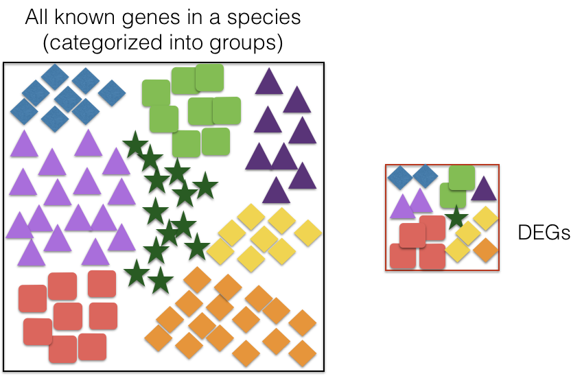
8.1.2 What is GO Enrichment Analysis?
GO enrichment analysis asks whether certain GO terms occur more often in your list of genes than expected by chance.
For example, if 10% of all genes in the genome are involved in “DNA repair,” but 30% of your up-regulated genes are, that process is enriched.
Statistical tests such as the hypergeometric test or Fisher’s exact test are used to determine whether this enrichment is significant.
In essence, GO enrichment helps you summarize large gene lists into meaningful biological patterns.
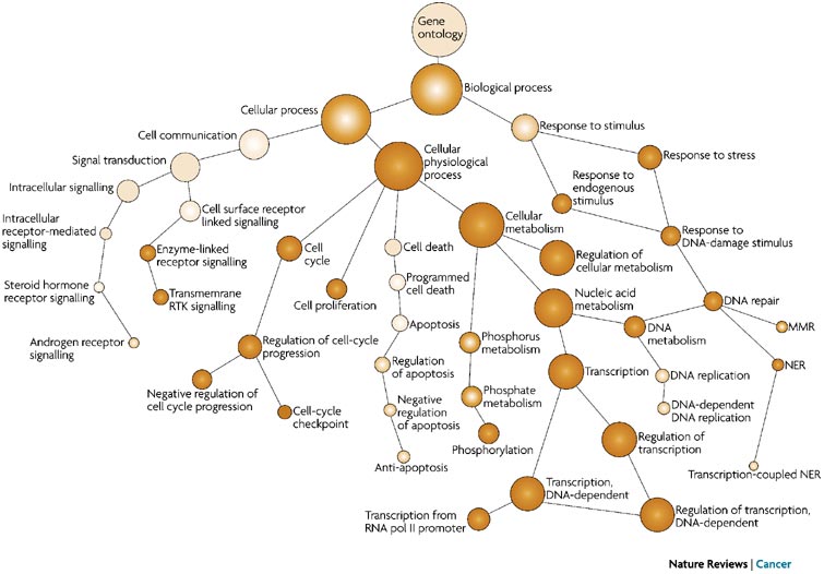
8.1.3 Ontology and GO Terms
Ontology: An ontology is a classification of things that are detectable or directly observable and the relationships between those things.
The Gene Ontology (GO) project provides an ontology of defined terms representing gene product properties. These terms are connected to each other via formally defined relationships, allowing for consistent annotation and analysis of gene functions across different species and research areas.
GO term hierarchy Some gene products are well-researched, with vast quantities of data available regarding their biological processes and functions. However, other gene products have very little data available about their roles in the cell.
For example, the protein, “p53”, would contain a wealth of information on it’s roles in the cell, whereas another protein might only be known as a “membrane-bound protein” with no other information available.
The GO ontologies were developed to describe and query biological knowledge with differing levels of information available. To do this, GO ontologies are loosely hierarchical, ranging from general, ‘parent’, terms to more specific, ‘child’ terms. The GO ontologies are “loosely” hierarchical since ‘child’ terms can have multiple ‘parent’ terms.
Some genes with less information may only be associated with general ‘parent’ terms or no terms at all, while other genes with a lot of information be associated with many terms.
8.1.4 GO Terms (Gene Ontology Terms)
The GO terms describe three aspects of gene products:
- Biological Process: Refers to the biological objectives achieved by gene products, such as “cell division” or “response to stress.” Inferred from Direct Assay (IDA)
Molecular Function: Describes the biochemical activities at the molecular level, such as “kinase activity” or “DNA binding.”
Cellular Component: Indicates where gene products are located within the cell, like “nucleus” or “mitochondrion.”
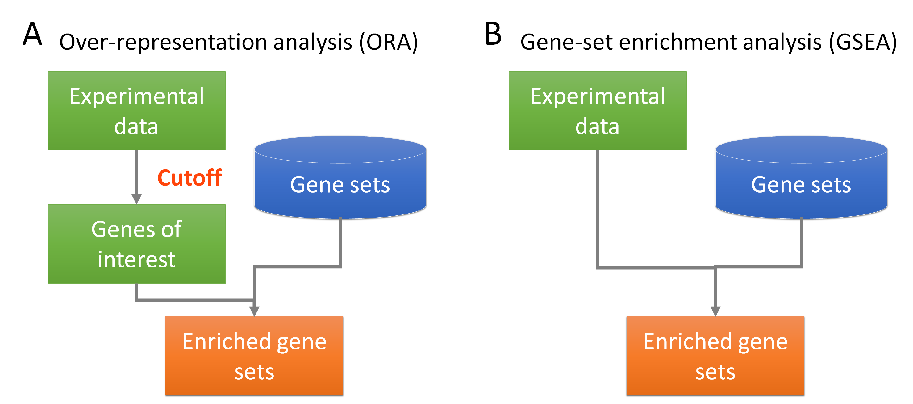
8.1.5 GO Enrichment Methods
GO enrichment methods help interpret differentially expressed gene lists from RNA-seq data and include the following:
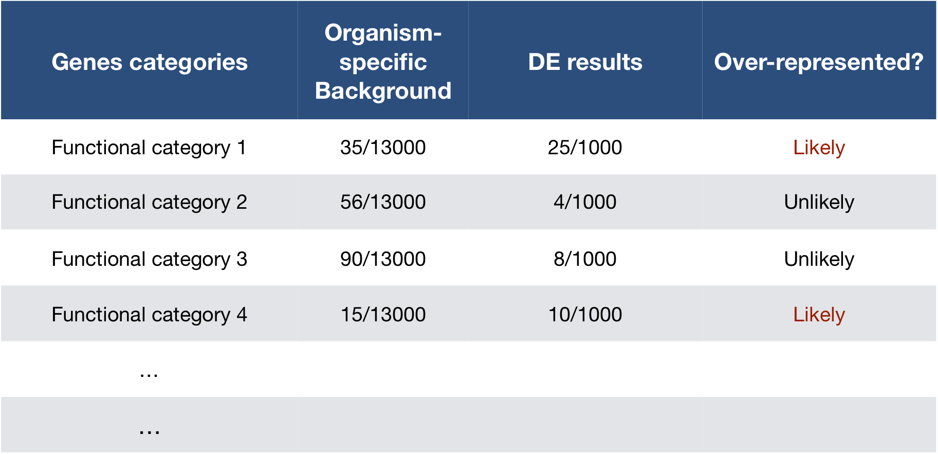
- Overrepresentation Analysis (ORA):
- ORA assesses whether specific GO terms are over-represented in a gene list compared to the background set of genes (e.g., all genes in the genome). Over-represented GO terms indicate biological functions or processes that are significantly associated with the genes of interest.
 `
`
- Hypergeometric Test:
The hypergeometric test in GO enrichment analysis is used to determine whether a set of genes is enriched for specific GO terms compared to the background set of genes. The test calculates the probability of observing the overlap between the query gene set and the gene set associated with a particular GO term, given the total number of genes in the dataset and the number of genes in the background set.
Test Analogy: The jar contains:
🔴 Red balls
⚫ Black balls
The hypergeometric test asks: “If I randomly drew this many balls from the jar, what’s the probability I’d get at least this many red balls just by chance?”
So, it’s like drawing colored balls from a jar where:
🔴 Red balls = genes that belong to a specific GO term
⚫ Black balls = genes that do NOT belong to that GO term
Total balls in jar = all genes in your background (universe)
You draw from the jar:
You draw a handful of balls = your significant genes (e.g., padj < 0.05)
The test checks how surprising it is that so many of your significant genes are red.
If the probability of getting that many red balls (GO term genes) by chance is very low, then the GO term is overrepresented — meaning your experiment is likely enriched for that biological process.
Note for the curious:
Click to see the mathematical formula
The hypergeometric test is based on counting combinations — the number of ways to draw q or more “successes” (genes with a given GO term) in k draws from a total of N genes, of which m belong to that GO term.
The formula for the cumulative probability of observing at least q successes (the upper-tail probability) in a sample of size \(k\) from a population with \(m\) successes and \(N - m\) failures is:
\[ P(X \geq q) = \sum_{i=q}^{k} \frac{\binom{m}{i} \binom{N - m}{k - i}}{\binom{N}{k}} \]
Where:
N: The total number of genes in the background set (e.g., all genes in the genome).m: The total number of genes in the background annotated with a specific GO term.k: The total number of genes in your gene list of interest.q: The number of genes in your list that are annotated with that specific GO term.
8.2 Perform the hypergeometric test: P(X >= q)
In R, the phyper() function computes the probability of observing this much overlap (or more) between our gene list and a GO term by chance.
Suppose your background population has \(N = 20,000\) genes (e.g., the entire genome). Out of these, \(m = 500\) genes are associated with a specific GO term (e.g., “cell cycle regulation”). You have a list of \(k = 1000\) genes of interest. In this list, \(q = 50\) genes are associated with the “cell cycle regulation” GO term.
A small p-value indicates that observing 50 or more genes with this GO term is unlikely by chance alone, suggesting genuine enrichment.
Question: Is 50 more than we’d expect by chance?
# Define parameters
N <- 20000         # Total genes in the background
m <- 500           # Genes with the GO term in background
k <- 1000          # Your gene list size (e.g., DE genes)
q <- 50            # Observed overlap with GO term

# Perform the hypergeometric test: P(X >= q)
# Note: We use q-1 because phyper calculates P(X > q-1) = P(X >= q)
p_value <- phyper(q - 1, m, N - m, k, lower.tail = FALSE)
p_value
## [1] 2.551199e-06A small p-value indicates that observing 50 or more genes with this GO term is unlikely by chance alone, suggesting genuine enrichment.
- Gene Set Enrichment Analysis (GSEA):
GSEA uses the entire ranked list of genes (ranked by log2FoldChange or similar metric) rather than just significant ones. It checks whether genes in a pathway tend to cluster at the top or bottom of your ranked list, indicating coordinated expression changes.
When to use each: - ORA: When you have clear significant genes (padj < 0.05) - GSEA: When you want to detect subtle coordinated changes across many genes
For this course, we’ll focus on Over-representation Analysis (ORA) which is more commonly used and straightforward to interpret.
8.3 Over-Representation Analysis (ORA)
We’ll explore ORA using two different R packages that use the same underlying statistical method (hypergeometric test) but offer different visualization capabilities.
8.3.1 Over-representation Analysis (ORA) using clusterProfiler
# Uncomment the following if you haven't yet installed either `GOenrichment` or `org.Hs.eg.db`
# devtools::install_github("gurinina/GOenrichment", force = TRUE)
#
# BiocManager::install("org.Hs.eg.db", force = TRUE)

## Load required libraries
library(org.Hs.eg.db)
library(clusterProfiler)
library(tidyverse)
library(enrichplot)
library(fgsea)
library(igraph)
library(ggraph)
library(visNetwork)
library(GO.db)
library(GOSemSim)
library(GOenrichment)
library(tidydr)
8.3.1.1 Running clusterProfiler: we first need to load the results of the differential expression analysis.
res_tableOE = readRDS("data/res_tableOE.RDS")

res_tableOE_tb <- res_tableOE %>%
  data.frame() %>% rownames_to_column(var = "gene") %>%
  dplyr::filter(!is.na(log2FoldChange))  %>% as_tibble()
To perform the over-representation analysis, we need a list of background genes and a list of significant genes:
## background set of genes
allOE_genes <- res_tableOE_tb$gene


sigOE = dplyr::filter(res_tableOE_tb, padj < 0.05) # Standard padj value

## significant genes
sigOE_genes = sigOE$geneTheenrichGO() function performs the ORA for the significant genes of interest (sigOE_genes) compared to the background gene list (allOE_genes) and returns the enriched GO terms and their associated p-values.
## Run GO enrichment analysis
ego <- enrichGO(gene = sigOE_genes,
 universe = allOE_genes,
 keyType = "SYMBOL",
 OrgDb = org.Hs.eg.db,
 minGSSize = 20,
 maxGSSize = 300,
 ont = "BP",
 pAdjustMethod = "BH",
 qvalueCutoff = 0.01,   # slightly stringent FDR cutoff
 readable = TRUE)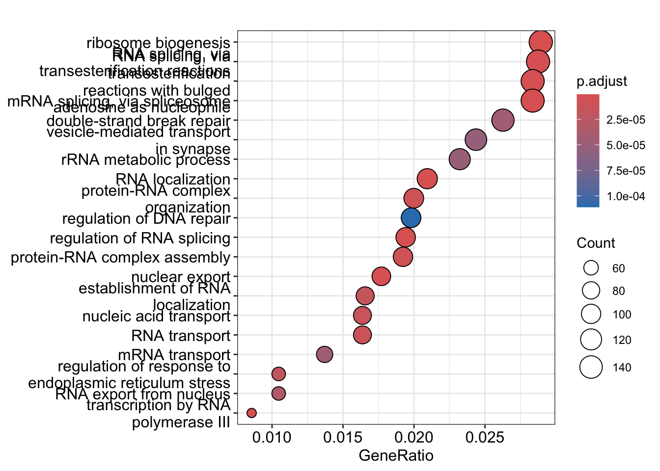
8.3.2 Visualizing GO Enrichment Results
After identifying enriched GO terms with enrichGO(), we can visualize the relationships between them using several complementary plots from clusterProfiler.
8.3.2.1 Network Plot with emapplot()
The emapplot() function creates a network where:
- Nodes represent GO terms
- Edges connect terms that share genes (calculated using Jaccard similarity)
- Clusters of connected nodes indicate related biological processes
This helps identify groups of functionally related processes affected in your experiment.
# Filter to top 50 most significant results for clearer visualization
ego_filtered <- ego
ego_filtered@result <- ego@result[1:50, ]  # Take only top 50 results

# Calculate pairwise term similarity based on gene overlap
# "JC" = Jaccard coefficient (size of intersection / size of union)
pwt_filtered <- pairwise_termsim(ego_filtered, method = "JC")

# Create network plot
emapplot(
  pwt_filtered,
  showCategory = 50,
  node_label = "category",
  layout = "mds"
) +
  theme(legend.position = "none")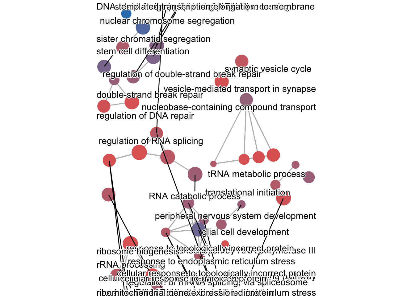
What to look for in the network:
- Clusters of connected nodes = related biological processes
- Isolated nodes = unique processes
- Edge thickness = strength of gene overlap between terms
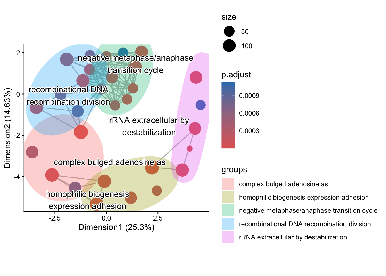
8.3.2.2 Overview with ssplot()
The ssplot() provides a simplified overview of the most significant terms and their relationships:
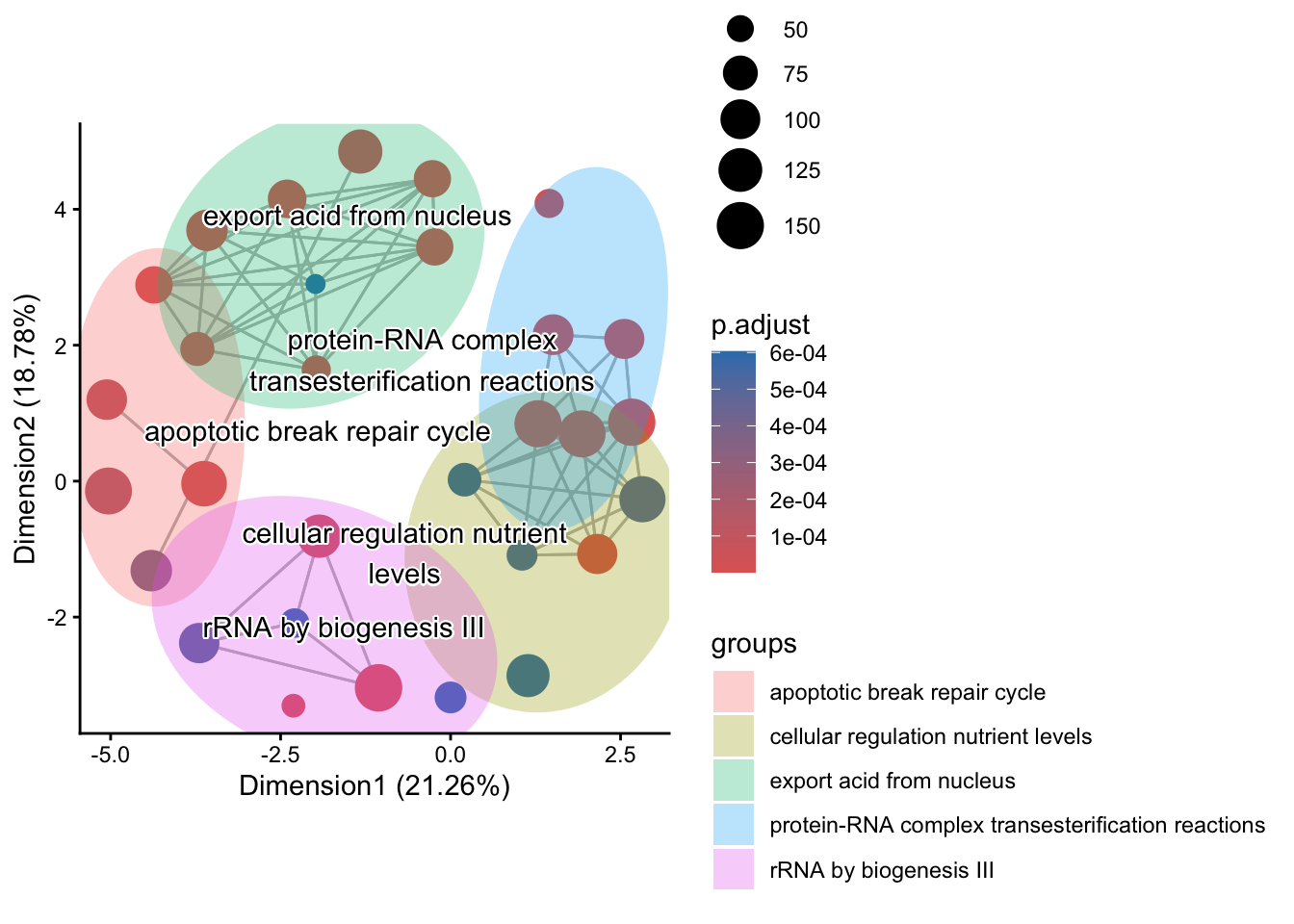
This plot gives you a cleaner, high-level view of term relationships compared to the detailed network above.
8.3.2.3 Gene-Concept Network with cnetplot()
The cnetplot() shows which specific genes belong to which GO terms. This is useful for identifying genes that may be key regulators involved in multiple biological processes:
cnetplot(pwt_filtered, showCategory = 3,
         categorySize = "pvalue",
         colorEdge = TRUE) +
  theme(legend.position = "none")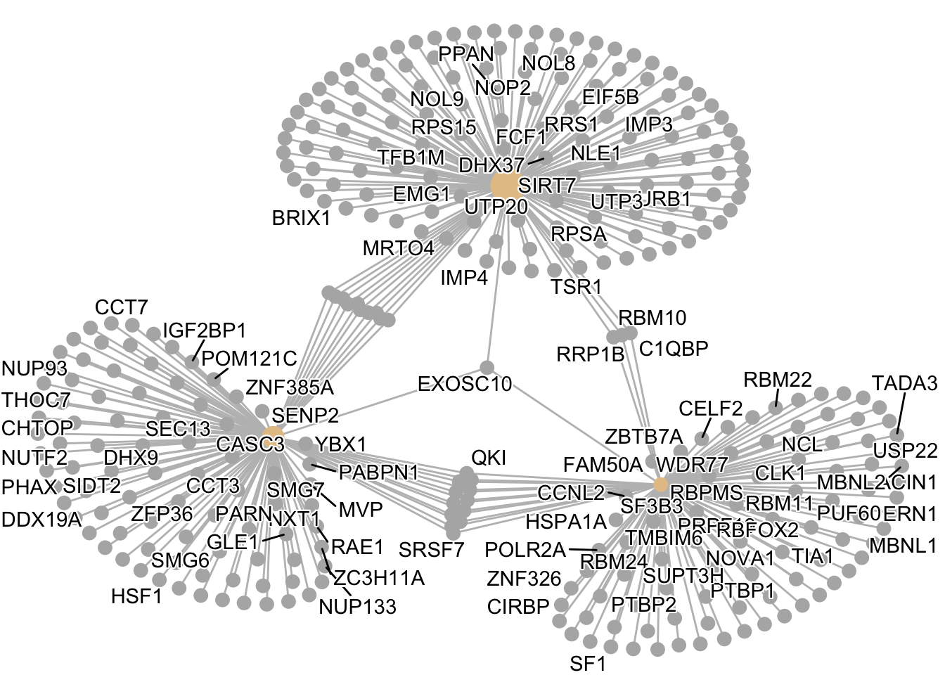
Interpretation: In this plot: - Large circles = GO terms (size shows significance) - Small circles = genes - Lines connect genes to their GO terms - Genes connected to multiple terms are potential hub genes affecting several processes
8.3.3 Comparing ORA Methods: enricher vs runGORESP
Now that we’ve seen ORA with clusterProfiler’s enrichGO(), let’s use another package called GOenrichment that performs the same hypergeometric test but adds interactive network visualization using visNetwork.
8.3.4 GOenrichment Package Analysis
We’re going to run this analysis using TWO different packages. Why? In research, you often want to verify important results using independent methods. We’ll see that both give us similar answers (~90% overlap), which builds confidence. They differ slightly because of minor implementation details, which is normal and expected.
runGORESP uses over-representation analysis to identify enriched GO terms and returns two data.frames; of enriched GO terms (nodes) and GO term relationships (edges). We first need to get the GO annotations and specifically ‘Biological Process’ (BP).
- Generate clean GO Biological Process gene sets with gene symbols
# install.packages("msigdbr") # uncomment to install
library(msigdbr)

# Using msigdbr ensures standardized, up-to-date gene sets
go_bp <- msigdbr(species = "Homo sapiens", collection = "C5", subcollection = "GO:BP")

# Let's look at the format of go_bp
names(go_bp)
## [1] "gene_symbol" "ncbi_gene" "ensembl_gene"
## [4] "db_gene_symbol" "db_ncbi_gene" "db_ensembl_gene"
## [7] "source_gene" "gs_id" "gs_name"
## [10] "gs_collection" "gs_subcollection" "gs_collection_name"
## [13] "gs_description" "gs_source_species" "gs_pmid"
## [16] "gs_geoid" "gs_exact_source" "gs_url"
## [19] "db_version" "db_target_species"| gene_symbol | gs_id |
|---|---|
| AASDHPPT | M29088 |
| ALDH1L1 | M29088 |
| ALDH1L2 | M29088 |
| MTHFD1 | M29088 |
| MTHFD1L | M29088 |
| MTHFD2L | M29088 |
## [1] 617648 20## $GOBP_10_FORMYLTETRAHYDROFOLATE_METABOLIC_PROCESS
## [1] "AASDHPPT" "ALDH1L1" "ALDH1L2" "MTHFD1" "MTHFD1L" "MTHFD2L"
##
## $GOBP_2_OXOGLUTARATE_METABOLIC_PROCESS
## [1] "AADAT" "ADHFE1" "COL6A1" "D2HGDH" "DLD" "DLST" "GOT1" "GOT2"
## [9] "GPT2" "IDH1" "IDH2" "KGD4" "KYAT3" "L2HGDH" "OGDH" "OGDHL"
## [17] "PHYH" "TAT"# Clean up term names (remove GOBP_ prefix and replace underscores)
names(hGOBP.gmt) <- gsub("^GOBP_", "", names(hGOBP.gmt))
names(hGOBP.gmt) <- gsub("_", " ", names(hGOBP.gmt))
hGOBP.gmt[1:2]## $`10 FORMYLTETRAHYDROFOLATE METABOLIC PROCESS`
## [1] "AASDHPPT" "ALDH1L1" "ALDH1L2" "MTHFD1" "MTHFD1L" "MTHFD2L"
##
## $`2 OXOGLUTARATE METABOLIC PROCESS`
## [1] "AADAT" "ADHFE1" "COL6A1" "D2HGDH" "DLD" "DLST" "GOT1" "GOT2"
## [9] "GPT2" "IDH1" "IDH2" "KGD4" "KYAT3" "L2HGDH" "OGDH" "OGDHL"
## [17] "PHYH" "TAT"Create GO ID (go_input argument) for runGORESP: assigns GO IDs to GO terms
go_mapping <- go_bp[!duplicated(go_bp$gs_name), c("gs_name", "gs_id")]


# Let's look at the format of go_mapping
head(go_mapping)| gs_name | gs_id |
|---|---|
| GOBP_10_FORMYLTETRAHYDROFOLATE_METABOLIC_PROCESS | M29088 |
| GOBP_2FE_2S_CLUSTER_ASSEMBLY | M23654 |
| GOBP_2_OXOGLUTARATE_METABOLIC_PROCESS | M15857 |
| GOBP_3_UTR_MEDIATED_MRNA_DESTABILIZATION | M24263 |
| GOBP_3_UTR_MEDIATED_MRNA_STABILIZATION | M11060 |
| GOBP_4FE_4S_CLUSTER_ASSEMBLY | M45874 |
names(go_mapping) <- c("term", "GOID")

# Cleanup GO terms
go_mapping$term <- gsub("^GOBP_", "", go_mapping$term)
go_mapping$term <- gsub("_", " ", go_mapping$term)

head(go_mapping)| term | GOID |
|---|---|
| 10 FORMYLTETRAHYDROFOLATE METABOLIC PROCESS | M29088 |
| 2FE 2S CLUSTER ASSEMBLY | M23654 |
| 2 OXOGLUTARATE METABOLIC PROCESS | M15857 |
| 3 UTR MEDIATED MRNA DESTABILIZATION | M24263 |
| 3 UTR MEDIATED MRNA STABILIZATION | M11060 |
| 4FE 4S CLUSTER ASSEMBLY | M45874 |
enricheruses over-representation analysis to identify enriched GO terms. Prepare data for enricher: Create TERM2GENE data frame (term = GO term, gene = gene symbol) for the GO library
| gs_name | gene_symbol |
|---|---|
| GOBP_10_FORMYLTETRAHYDROFOLATE_METABOLIC_PROCESS | AASDHPPT |
| GOBP_10_FORMYLTETRAHYDROFOLATE_METABOLIC_PROCESS | ALDH1L1 |
| GOBP_10_FORMYLTETRAHYDROFOLATE_METABOLIC_PROCESS | ALDH1L2 |
| GOBP_10_FORMYLTETRAHYDROFOLATE_METABOLIC_PROCESS | MTHFD1 |
| GOBP_10_FORMYLTETRAHYDROFOLATE_METABOLIC_PROCESS | MTHFD1L |
| GOBP_10_FORMYLTETRAHYDROFOLATE_METABOLIC_PROCESS | MTHFD2L |
names(term2gene) <- c("term", "gene")

# Cleanup GO terms
term2gene$term <- gsub("^GOBP_", "", term2gene$term)
term2gene$term <- gsub("_", " ", term2gene$term)

head(term2gene)| term | gene |
|---|---|
| 10 FORMYLTETRAHYDROFOLATE METABOLIC PROCESS | AASDHPPT |
| 10 FORMYLTETRAHYDROFOLATE METABOLIC PROCESS | ALDH1L1 |
| 10 FORMYLTETRAHYDROFOLATE METABOLIC PROCESS | ALDH1L2 |
| 10 FORMYLTETRAHYDROFOLATE METABOLIC PROCESS | MTHFD1 |
| 10 FORMYLTETRAHYDROFOLATE METABOLIC PROCESS | MTHFD1L |
| 10 FORMYLTETRAHYDROFOLATE METABOLIC PROCESS | MTHFD2L |
- Run
enricheranalysis:
# Optimal parameters for robust analysis
enricher_result <- enricher(
    gene = sigOE_genes,
    TERM2GENE = term2gene,
    pvalueCutoff = 1,
    qvalueCutoff = 0.0001,        # Stringent FDR threshold
    minGSSize = 20,               # Robust minimum size
    maxGSSize = 300
)- Prepare data for runGORESP
Create
scoreMat: data frame with gene, score, and index columns
# Filter to only include genes that have GO annotations
all_genes <- unique(term2gene$gene)
sigOE_genes <- sigOE_genes[sigOE_genes %in% all_genes]


# Now create scoreMat with the filtered gene lists
scoreMat <- data.frame(
    gene = all_genes,
    score = runif(length(all_genes)),      # Random scores
    index = ifelse(all_genes %in% sigOE_genes, 1, 0),  # 1 = gene of interest
    stringsAsFactors = FALSE
)

head(scoreMat)| gene | score | index |
|---|---|---|
| AASDHPPT | 0.5325493 | 1 |
| ALDH1L1 | 0.1054283 | 1 |
| ALDH1L2 | 0.7344826 | 1 |
| MTHFD1 | 0.6285584 | 1 |
| MTHFD1L | 0.2830434 | 1 |
| MTHFD2L | 0.6896176 | 0 |
## [1] 18000 3## [1] 18000## [1] 5037##
## 0 1
## 12963 5037- Run
runGORESPanalysis:
goresp_result <- runGORESP(
    scoreMat = scoreMat,
    bp_input = hGOBP.gmt,                  # Gene sets as named list
    go_input = go_mapping,                 # GO term to ID mapping
    fdrThresh = 0.0001,                    # FDR threshold (same as enricher)
    minSetSize = 20,                       # Same as enricher minGSSize
    maxSetSize = 300                       # Same as enricher maxGSSize
)

names(goresp_result$edgeMat)
## [1] "source" "target" "overlapCoeff" "width" "label"## [1] "filename" "GOID" "term"
## [4] "nGenes" "nQuery" "nOverlap"
## [7] "querySetFraction" "geneSetFraction" "foldEnrichment"
## [10] "P" "FDR" "overlapGenes"
## [13] "maxOverlapGeneScore" "cluster" "id"
## [16] "size" "formattedLabel"| GOID | term | nGenes | nQuery | P |
|---|---|---|---|---|
| M16023 | RNA LOCALIZATION | 204 | 4998 | 0 |
| M16816 | REGULATION OF RNA SPLICING | 189 | 5150 | 0 |
| M24840 | VESICLE MEDIATED TRANSPORT IN SYNAPSE | 260 | 5117 | 0 |
| M15413 | NUCLEAR EXPORT | 172 | 5112 | 0 |
| M15304 | STEM CELL DIFFERENTIATION | 265 | 5003 | 0 |
| M23968 | ESTABLISHMENT OF RNA LOCALIZATION | 165 | 5115 | 0 |
## [1] 59 5## [1] 57 17- Display top results from both methods
##
## === Top enricher results ===## Description
## RNA LOCALIZATION RNA LOCALIZATION
## REGULATION OF RNA SPLICING REGULATION OF RNA SPLICING
## VESICLE MEDIATED TRANSPORT IN SYNAPSE VESICLE MEDIATED TRANSPORT IN SYNAPSE
## NUCLEAR EXPORT NUCLEAR EXPORT
## ESTABLISHMENT OF RNA LOCALIZATION ESTABLISHMENT OF RNA LOCALIZATION
## STEM CELL DIFFERENTIATION STEM CELL DIFFERENTIATION
## Count pvalue qvalue
## RNA LOCALIZATION 110 4.417655e-15 1.053727e-11
## REGULATION OF RNA SPLICING 103 1.293937e-14 1.543190e-11
## VESICLE MEDIATED TRANSPORT IN SYNAPSE 128 2.315881e-13 1.841329e-10
## NUCLEAR EXPORT 92 1.404827e-12 8.377206e-10
## ESTABLISHMENT OF RNA LOCALIZATION 87 1.573398e-11 7.345982e-09
## STEM CELL DIFFERENTIATION 125 1.847842e-11 7.345982e-09##
## === Top runGORESP results ===## term nOverlap P FDR
## 1 RNA LOCALIZATION 110 4.42e-15 1.48e-11
## 2 REGULATION OF RNA SPLICING 103 1.29e-14 2.17e-11
## 3 VESICLE MEDIATED TRANSPORT IN SYNAPSE 128 2.32e-13 2.59e-10
## 4 NUCLEAR EXPORT 92 1.40e-12 1.18e-09
## 5 STEM CELL DIFFERENTIATION 125 1.85e-11 1.03e-08
## 6 ESTABLISHMENT OF RNA LOCALIZATION 87 1.57e-11 1.03e-08## [1] 65 12## [1] 57 17- Let’s check the overlap between the enriched terms found using
runGORESPand those found usingenricheras they used the same GO term libraries:
overlap_terms <- intersect(enricher_result$ID, goresp_result$enrichInfo$term)
cat("Overlapping terms:", length(overlap_terms), "\n")
## Overlapping terms: 57cat("Overlap percentage:", round(100 * length(overlap_terms) /
max(nrow(enricher_result), nrow(goresp_result$enrichInfo)), 1), "%\n")## Overlap percentage: 87.7 %Percent overlap is close to 90% that is very good.
Key differences between methods - Both use hypergeometric testing with Benjamini-Hochberg FDR correction - enricher: Standard clusterProfiler workflow - runGORESP: Adds gene set clustering and network visualization features - Expected difference: 5-15% due to minor implementation differences - Core significant results are nearly identical
We can visualize the results of the runGORESP analysis using the visNetwork package. This package allows us to create interactive network visualizations.
We use thevisSetup function to prepare the data for network visualization. We then run the runNetwork function to generate the interactive network plot.
vis = visSetup(goresp_result$enrichInfo,goresp_result$edgeMat)
GOenrichment::runNetwork(vis$nodes, vis$edges, main = "MOV10 OE GO Enrichment Network")
This network analysis is based on Cytoscape, an open source bioinformatics software platform for visualizing molecular interaction networks from Gary Bader at the University of Toronto.
Exercise points = +4
1. Perform a GO enrichment analysis using the runGORESP function from the GOenrichment package using res_tableKD with a padj cutoff of 0.05. Use a significance FDR threshold of 0.0001. Save the results in a variable called kresp.
- Visualize the enriched GO terms using the
runNetworkfunction from theGOenrichmentpackage. Save the visualization setup in a variable calledkvis.
Solution
Step 1: Load and prepare the knockdown data
# Load the knockdown differential expression results
res_tableKD <- readRDS("data/res_tableKD.RDS")

# Convert to tibble and filter out genes with NA log2FoldChange
res_tableKD_tb <- res_tableKD %>%
  data.frame() %>%
  rownames_to_column(var = "gene") %>%
  dplyr::filter(!is.na(log2FoldChange)) %>%
  as_tibble()

# Identify significant genes using padj < 0.05
sigKD <- dplyr::filter(res_tableKD_tb, padj < 0.05)

# Extract significant gene names
sigKD_genes <- sigKD$gene

# Check how many significant genes we have
cat("Number of significant genes:", length(sigKD_genes), "\n")
## Number of significant genes: 4909Step 2: Prepare the score matrix for runGORESP
# Get all genes from the GO gene sets (already created earlier)
all_genes <- unique(go_bp$gene_symbol)

# Create score matrix
# The 'index' column marks which genes are significant (1) vs background (0)
scoreMat_kd <- data.frame(
    gene = all_genes,
    score = runif(length(all_genes)),      # Random scores (not used for ORA)
    index = ifelse(all_genes %in% sigKD_genes, 1, 0),  # 1 = significant gene
    stringsAsFactors = FALSE
)

# Check the score matrix
head(scoreMat_kd)| gene | score | index |
|---|---|---|
| AASDHPPT | 0.8466548 | 1 |
| ALDH1L1 | 0.3358286 | 0 |
| ALDH1L2 | 0.1377130 | 1 |
| MTHFD1 | 0.0455170 | 0 |
| MTHFD1L | 0.3843954 | 0 |
| MTHFD2L | 0.3779148 | 0 |
## Total genes in score matrix: 18000## Significant genes marked: 3890Step 3: Run GO enrichment analysis with runGORESP
# Run runGORESP with FDR threshold of 0.0001
kresp <- runGORESP(
    scoreMat = scoreMat_kd,
    bp_input = hGOBP.gmt,                  # GO gene sets (created earlier)
    go_input = go_mapping,                 # GO term to ID mapping (created earlier)
    fdrThresh = 0.0001,                    # Stringent FDR threshold
    minSetSize = 20,                       # Minimum genes in a GO term
    maxSetSize = 300                       # Maximum genes in a GO term
)

# Examine the results
cat("Number of enriched GO terms:", nrow(kresp$enrichInfo), "\n")
## Number of enriched GO terms: 45| term | nOverlap | P | FDR |
|---|---|---|---|
| EPITHELIAL CELL DEVELOPMENT | 96 | 0 | 0e+00 |
| TELENCEPHALON DEVELOPMENT | 111 | 0 | 0e+00 |
| PROTEIN LOCALIZATION TO PLASMA MEMBRANE | 113 | 0 | 1e-07 |
| RNA LOCALIZATION | 85 | 0 | 1e-07 |
| REGULATION OF MICROTUBULE CYTOSKELETON ORGANIZATION | 74 | 0 | 1e-07 |
| SPINDLE ORGANIZATION | 84 | 0 | 6e-07 |
Step 4: Create interactive network visualization
8.4 Gene Set Enrichment Analysis (GSEA) - Optional
Note: This section is optional. GSEA uses all ranked genes rather than just significant ones. We’ll focus on ORA in this course, but GSEA is shown here for reference.
8.4.1 GSEA Using ‘clusterProfiler’ `gseGO’
Prepare fold changes, sort by expression, and run GSEA with gseGO() from clusterProfiler
## Extract the foldchanges
foldchanges <- res_tableOE_tb$log2FoldChange

## Name each fold change with the gene name
names(foldchanges) <- res_tableOE_tb$gene

## Sort fold changes in decreasing order
foldchanges <- sort(foldchanges, decreasing = TRUE)
We can use GSEA to test whether genes in specific biological processes tend to be up- or down-regulated together in our experiment:
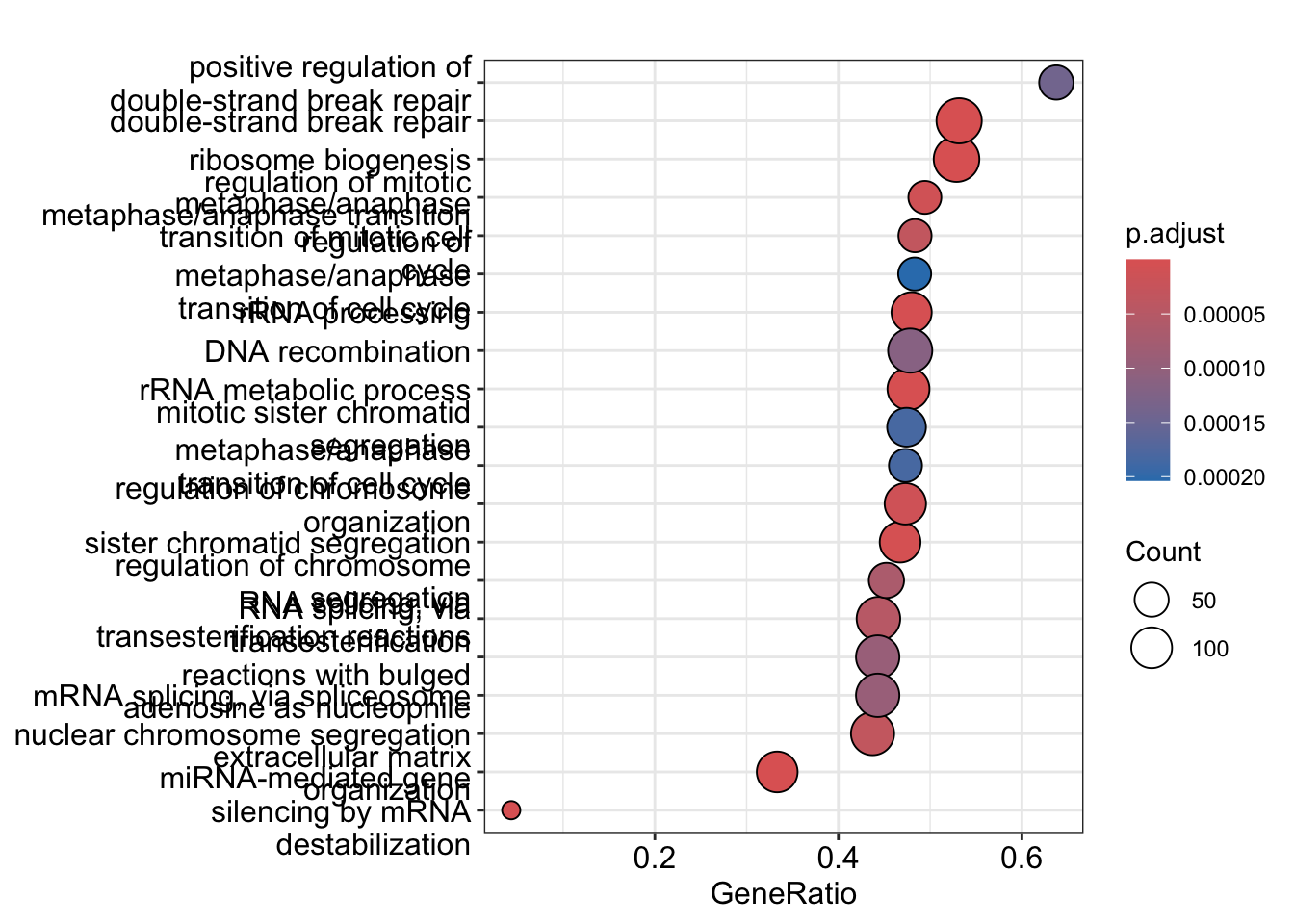
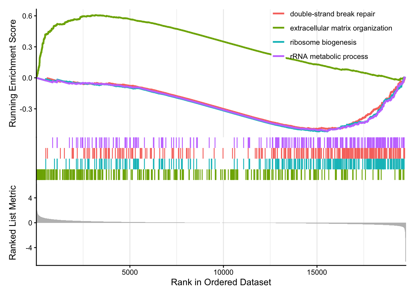
8.4.2 Visualizing GSEA Results
Visualize GSEA results with dotplot() for significant categories and gseaplot2() for gene set ranks.
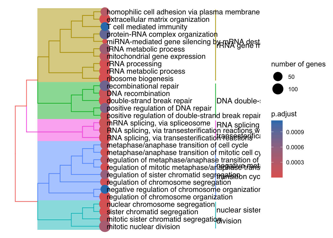
The emapplot clusters the 50 most significant (by padj) GO terms to visualize relationships between terms.
gseaGO_filtered <- gseaGO
gseaGO_filtered@result <- gseaGO@result[1:50, ]  # Top 50 by p.adjust

# Create pairwise similarity
pwt <- pairwise_termsim(
  gseaGO_filtered,
  method = "JC",
  semData = NULL
)


emapplot(pwt, showCategory = 50,
node_label = "category") 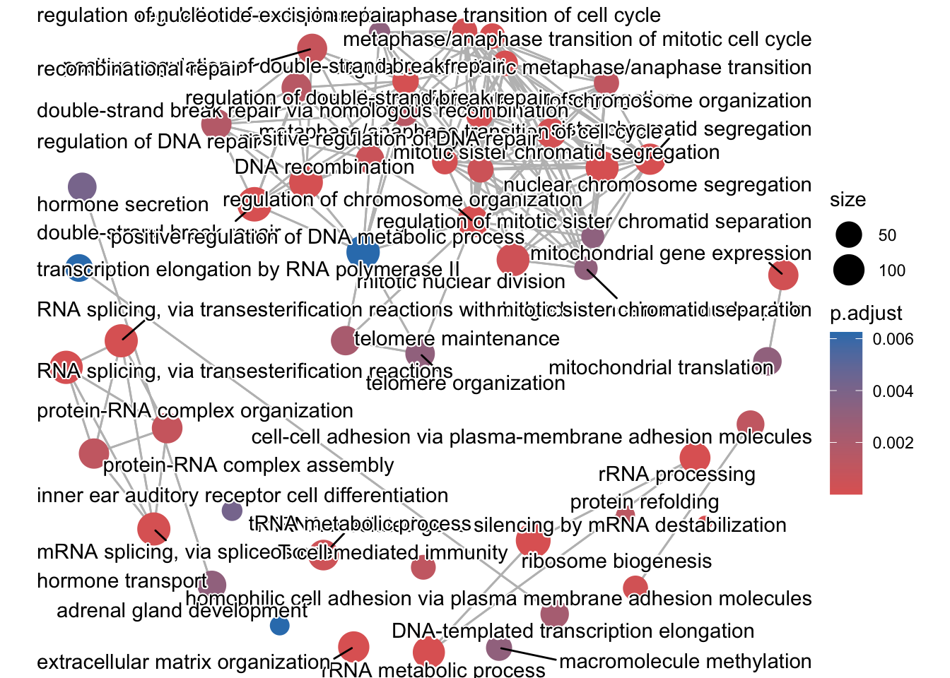
We are going to compare ORA enricher to running the ORA runGORESP.
Let’s first load the GOenrichment package:
# Uncomment the following if you haven't yet installed GOenrichment.

# devtools::install_github("gurinina/GOenrichment")

library(GOenrichment)
8.4.3 Other tools and resources
GeneMANIA. GeneMANIA finds other genes that are related to a set of input genes, using a very large set of functional association data curated from the literature.
ReviGO. Revigo is an online GO enrichment tool that allows you to copy-paste your significant gene list and your background gene list. The output is a visualization of enriched GO terms in a hierarchical tree.
AmiGO. AmiGO is the current official web-based set of tools for searching and browsing the Gene Ontology database.
etc.