Chapter 4 Differential expression analysis with DESeq2
The final step in the differential expression analysis workflow is fitting the raw counts to the NB model and performing the statistical test for differentially expressed genes. In this step we essentially want to determine whether the mean expression levels of different sample groups are significantly different.
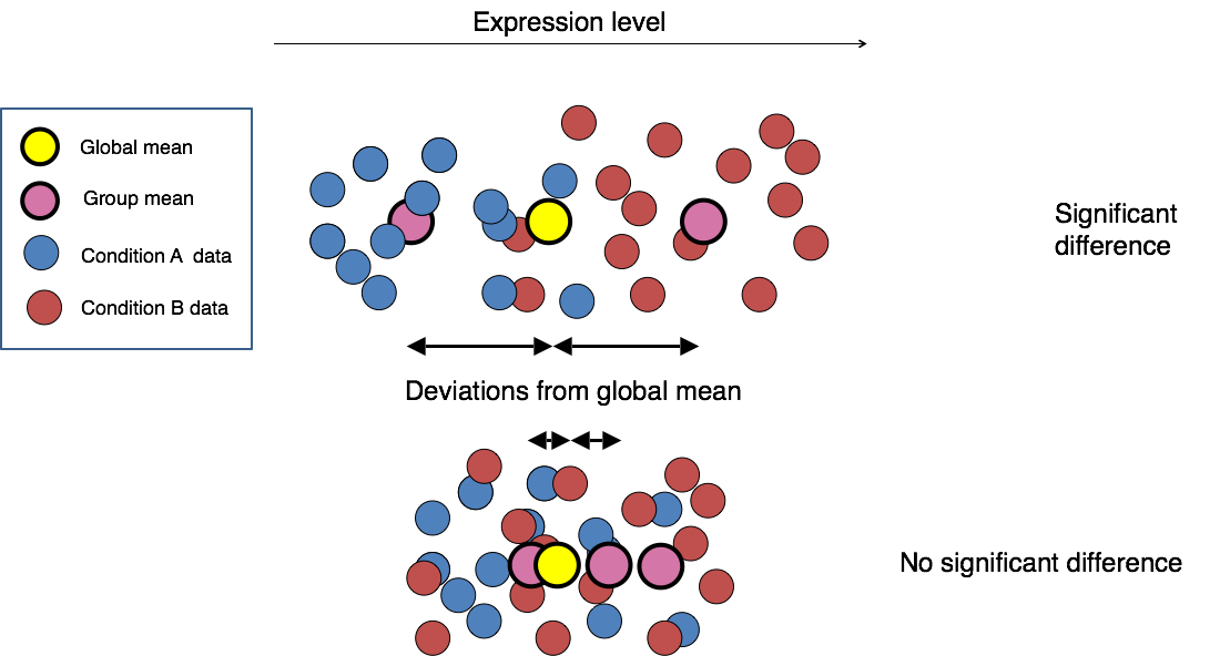
Image credit: Paul Pavlidis, UBC
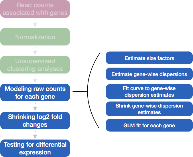
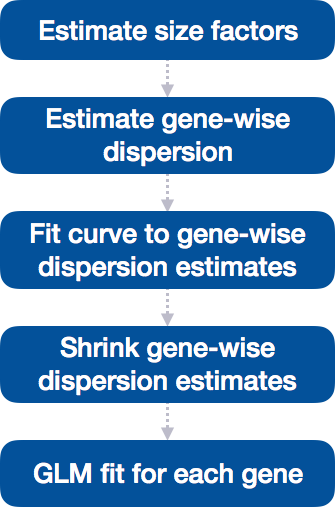
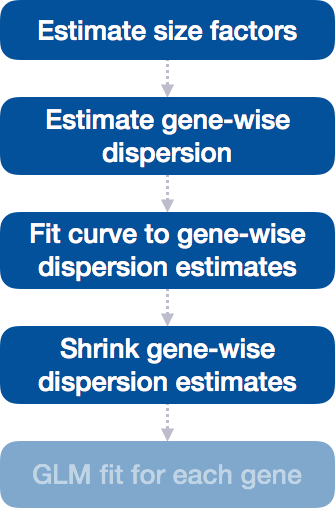
Differential expression analysis with DESeq2 involves multiple steps as displayed in the flowchart below in blue. Briefly, DESeq2 will model the raw counts, using normalization factors (size factors) to account for differences in library depth. Then, it will estimate the gene-wise dispersions and shrink these estimates to generate more accurate estimates of dispersion to model the counts. Finally, DESeq2 will fit the negative binomial model and perform hypothesis testing using the Wald test or Likelihood Ratio Test.
4.1 Running DESeq2
Prior to performing the differential expression analysis, it is a good idea to know what sources of variation are present in your data, either by exploration during the QC and/or prior knowledge. Once you know the major sources of variation, you can control for them in the statistical model by including them in your design formula.
4.1.1 Design formula
A design formula tells the statistical software the known sources of variation to control for, as well as, the factor of interest to test for during differential expression testing. For example, if you know that sex is a significant source of variation in your data, then sex should be included in your model. The design formula should have all of the factors in your metadata that account for major sources of variation in your data. The last factor entered in the formula should be the condition of interest.
For example, suppose you have the following metadata:
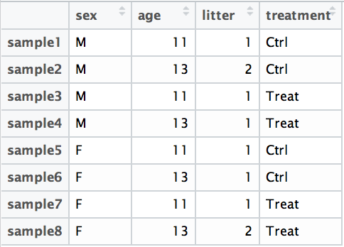
If you want to examine the expression differences between treatments, and you know that major sources of variation include sex and age, then your design formula would be:
design <- ~ sex + age + treatment
The tilde (~) should always proceed your factors and tells DESeq2 to model the counts using the following formula. Note the factors included in the design formula need to match the column names in the metadata.
Exercise points = +3
- Suppose you wanted to study the expression differences between the two age groups in the metadata shown above, and major sources of variation were
sexandtreatment, how would the design formula be written?
# the default behavior of `results` is to return the comparison of the last group in the design formula, so your condition of interest should come last.Based on our Mov10 metadata dataframe, which factors could we include in our design formula?
What would you do if you wanted to include a factor in your design formula that is not in your metadata?
4.1.2 MOV10 Differential Expression Analysis
Running Differential Expression in Two Lines of Code
To obtain differential expression results from our raw count data, we only need to run two lines of code!
First, we create a DESeqDataSet, as we did in the ‘Count normalization’ lesson, specifying the location of our raw counts and metadata, and applying our design formula:
## Create DESeq object
dds <- DESeqDataSetFromMatrix(countData = data, colData = meta, design = ~ sampletype)
Next, we run the actual differential expression analysis with a single call to the DESeq() function. This function handles everything—from normalization to linear modeling—all in one step. During execution, DESeq2 will print messages detailing the steps being performed: estimating size factors, estimating dispersions, gene-wise dispersion estimates, modeling the mean-dispersion relationship, and statistical testing for differential expression.
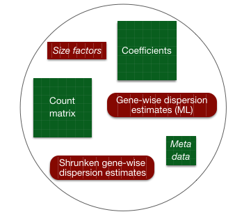
By re-assigning the result to back to the same variable name (dds), we update our DESeqDataSet object, which will now contain the results of each step in the analysis, effectively filling in the slots of our DESeqDataSet object.
4.1.3 DESeq2 differential gene expression analysis workflow
Everything from normalization to linear modeling was carried out by the use of a single function!
With the 2 lines of code above, we just completed the workflow for the differential gene expression analysis with DESeq2. The steps in the analysis are output below:
Everything from normalization to linear modeling was carried out by the use of a single function! This function will print out a message for the various steps it performs:
estimating size factors
estimating dispersions
gene-wise dispersion estimates
mean-dispersion relationship
final dispersion estimates
fitting model and testing
NOTE: There are individual functions available in DESeq2 that would allow us to carry out each step in the workflow in a step-wise manner, rather than a single call. We demonstrated one example when generating size factors to create a normalized matrix. By calling
DESeq()the individual functions for each step are run for you.
4.2 DESeq2 differential gene expression analysis workflow
With the 2 lines of code above, we just completed the workflow for the differential gene expression analysis with DESeq2. The steps in the analysis are output below:
We will be taking a detailed look at each of these steps to better understand how DESeq2 is performing the statistical analysis and what metrics we should examine to explore the quality of our analysis.
4.2.1 Step 1: Estimate size factors
The first step in the differential expression analysis is to estimate the size factors, which is exactly what we already did to normalize the raw counts.
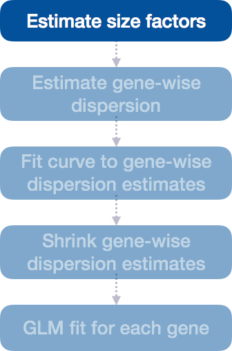
DESeq2 will automatically estimate the size factors when performing the differential expression analysis. However, if you have already generated the size factors using estimateSizeFactors(), as we did earlier, then DESeq2 will use these values.
4.2.1.1 MOV10 DE analysis: examining the size factors
Let’s take a quick look at size factor values we have for each sample:
## Irrel_kd_1 Irrel_kd_2 Irrel_kd_3 Mov10_kd_2 Mov10_kd_3 Mov10_oe_1 Mov10_oe_2
##  1.1224020  0.9625632  0.7477715  1.5646728  0.9351760  1.2016082  1.1205912
## Mov10_oe_3
##  0.6534987
These numbers should be identical to those we generated initially when we had run the function estimateSizeFactors(dds).
Exercise points = +2
Take a look at the total number of reads for each sample:
## Irrel_kd_1 Irrel_kd_2 Irrel_kd_3 Mov10_kd_2 Mov10_kd_3 Mov10_oe_1 Mov10_oe_2
##   22687366   19381680   14962754   32826936   19360003   23447317   21713289
## Mov10_oe_3
##   12737889
How do the numbers correlate with the size factor?
Now take a look at the total depth after normalization using:
## Irrel_kd_1 Irrel_kd_2 Irrel_kd_3 Mov10_kd_2 Mov10_kd_3 Mov10_oe_1 Mov10_oe_2
##   20213226   20135487   20009794   20980064   20701989   19513279   19376636
## Mov10_oe_3
##   19491836
How do the normalized values across samples compare with the total counts taken for each sample?
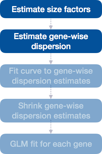
4.2.2 Step 2: Estimate gene-wise dispersion
DESeq2 estimates dispersion for each gene - a measure of how much gene expression varies between biological replicates. DESeq2’s dispersion parameter is specifically designed for this. It tells you after accounting for the mean-variance relationship in count data, how variable is this gene? High dispersion genes are legitimately noisy (biologically or technically), regardless of expression level.
Models variance as:
\[\text{Var}(Y_{ij}) = \mu_{ij} + \alpha_i \mu_{ij}^2\]
OR
\[\alpha = \frac{\text{Var}(Y) - \mu}{\mu^2}\]
Key pattern observed in RNA-seq data:
Low-expression genes tend to be more variable between replicates (higher dispersion)
High-expression genes tend to be more consistent between replicates (lower dispersion)
Why this matters: With only a few replicates per group, individual gene dispersion estimates can be noisy and unreliable. DESeq2 improves these estimates by using information from all genes, assuming that genes with similar expression levels should have similar variability using a statistical method called maximum likelihood estimation (MLE). In other words, given the count values of the replicates, the most likely estimate of dispersion is calculated.
4.2.3 Step 3: Fit Curve to Gene-wise Dispersion Estimates
After estimating gene-wise dispersions, DESeq2 fits a smooth curve of dispersion vs. mean expression across all genes.
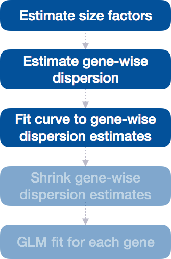
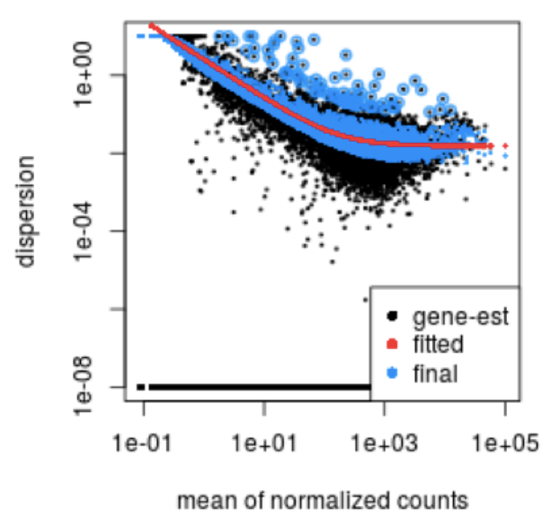
This curve is displayed as a red line in the figure below, which plots the estimate for the expected dispersion value for genes of a given expression strength. Each black dot is a gene with an associated mean expression level and maximum likelihood estimation (MLE) of the dispersion.
4.2.4 Step 4: Shrink gene-wise dispersion estimates toward the values predicted by the curve
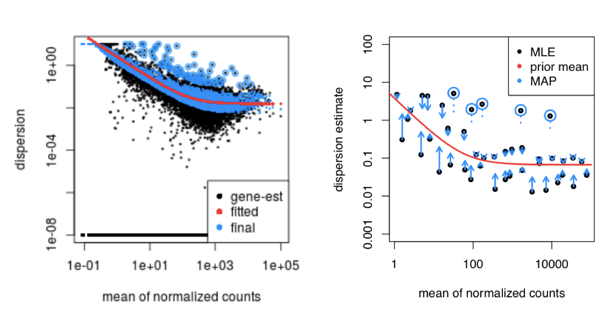
DESeq2 then “shrinks” each gene’s noisy estimate toward this curve. Genes with unreliable estimates (low counts) get adjusted more, while genes with reliable estimates (high counts) stay closer to their original values.
This shrinkage method is particularly important to reduce false positives in the differential expression analysis. Genes with low dispersion estimates are shrunken towards the curve, and the more accurate, higher shrunken values are output for fitting of the model and differential expression testing.
Dispersion estimates that are slightly above the curve are also shrunk toward the curve for better dispersion estimation; however, genes with extremely high dispersion values are not. This is due to the likelihood that the gene does not follow the modeling assumptions and has higher variability than others for biological or technical reasons. Shrinking the values toward the curve could result in false positives, so these values are not shrunken. These genes are shown surrounded by blue circles below.
This entire dispersion estimation and shrinkage process happens automatically when you run DESeq(dds).
4.2.5 MOV10 Differential Expression Analysis: Exploring Dispersion Estimates
Now, let’s explore the dispersion estimates for the MOV10 dataset:
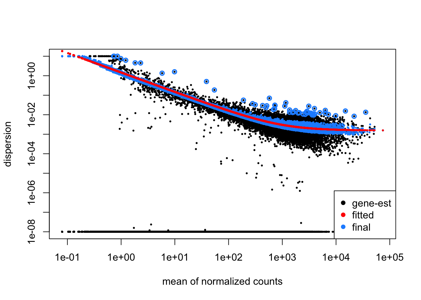 You should see genes scattered around a decreasing curve, with dispersion decreasing as mean expression increases. Since we have a small sample size, many genes show shrinkage toward the fitted trend (red line), which is expected and beneficial for the analysis.
Exercise points = +1
Do you think our data are a good fit for the model?