6 Optimization

Many, if not all projects in applied science and industry can be stated as constrained optimization problems. Given a K-dimensional cost function cost=f(x₁,x₂,…x_K) and some functionality, product or customer requirements y_j=g_j(x₁,x₂,…x_K), y_l=g_l(x₁,x₂,…x_K) the goal is finding optimal solutions (conditions) \(X^* =x_{1}^*,x_{2}^*,...x_{K}^*\) satisfying the functionality, product or customer requirements at minimal costs. In the optimization task, formula (6.1), LB_j and UB_j denote the lower and upper bounds of the quality targets while C_l are the targets that must be met exactly in the optimal solution.

\[\begin{gather} \min_{X} \big (cost=f(x_{1},x_{2},...x_{K}) \big ) \notag \\ subject \ to \notag \\ LB_{j} \leq y_{j} = g_{j}(x_{1},x_{2},...x_{K}) \leq UB_{j} \notag \\y_{l}=g_{l}(x_{1},x_{2},...x_{K}) = C_{l} \tag{6.1} \end{gather}\]

With all functional elements in the optimization problem, (6.1), analytically known, the problem can be solved using a mathematical optimizer - a piece of sophisticated software - as schematically depicted in figure 6.1. Of course, there is no guarantee that a solution will be found, as the problem might be infeasible⁴⁴ and conditions meeting the constraints cannot be found.

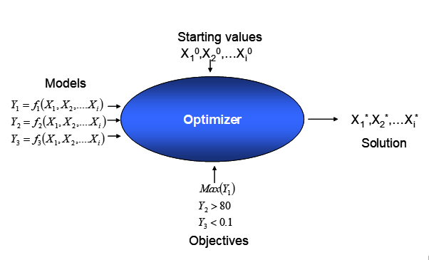
Figure 6.1: Solving a constrained optimization problem with mathematical optimization

A major obstacle in many applied projects is that analytical expressions g_j(x₁,x₁,…x_K) are not available or very laborious and expensive to obtain based on first principles, which makes a direct optimization approach inaccessible. However, DoE can be used to empirically derive surrogates of the true, however unknown functions y_j=g_j(x₁,x₂,…x_K) in the domain X and to derive local directions of ascend or descend depending on the optimization task. Optimization provides many techniques for navigating through high-dimensional space, some of which will be outlined in the following sections.

6.1 Non-linear functions

Non-linear and multidimensional functions can be divided into convex and non-convex functions with the former comparatively “easy” and the latter “hard” to optimize. Informally, a function is called convex, when all pairs of points on the function’s graph can be connected by a straight line without intersecting the function’s graph. When this property is lacking the function is called non-convex. This property is schematically depicted in figure 6.2.

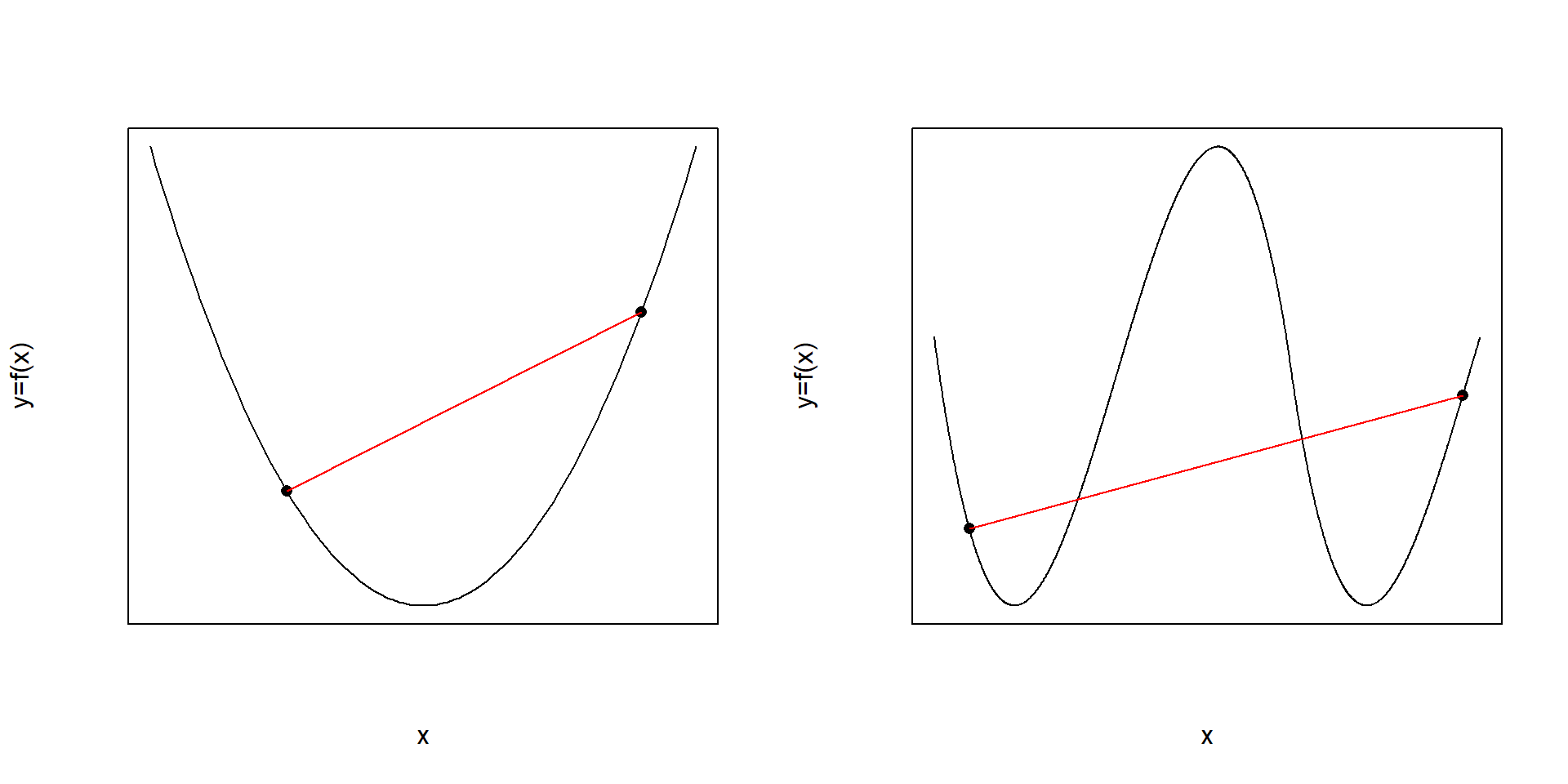
Figure 6.2: Convex (left panel) and non-convex (right panel) functions. Non-convexity on the right panel always imply some pairs of points on the graph which cannot be connected without intersecting the functions graph.

Convex functions have, as a direct consequence of these properties, one and only one extremum (or put differently: are twice continuously differentiable) while non-convex functions have several extrema (e.g., three in fig. 6.2, two minima and one maximum). This situation extends to high-dimensional space as the two-dimensional example function, figure 6.3, may indicate. Again, there can be several extrema (maxima, minima and additionally sattle points) and the function may reveal non-smooth domains with the function value changing abruptly in a phase transition like manner (of course, this can also apply to one-dimensional functions y=f(x)). Trying to optimize such functions with global optimization methods can be a nightmare and there is no guarantee that the gobal extremum (e.g. in figure 6.3: the maximum of all maxima) is found⁴⁵.

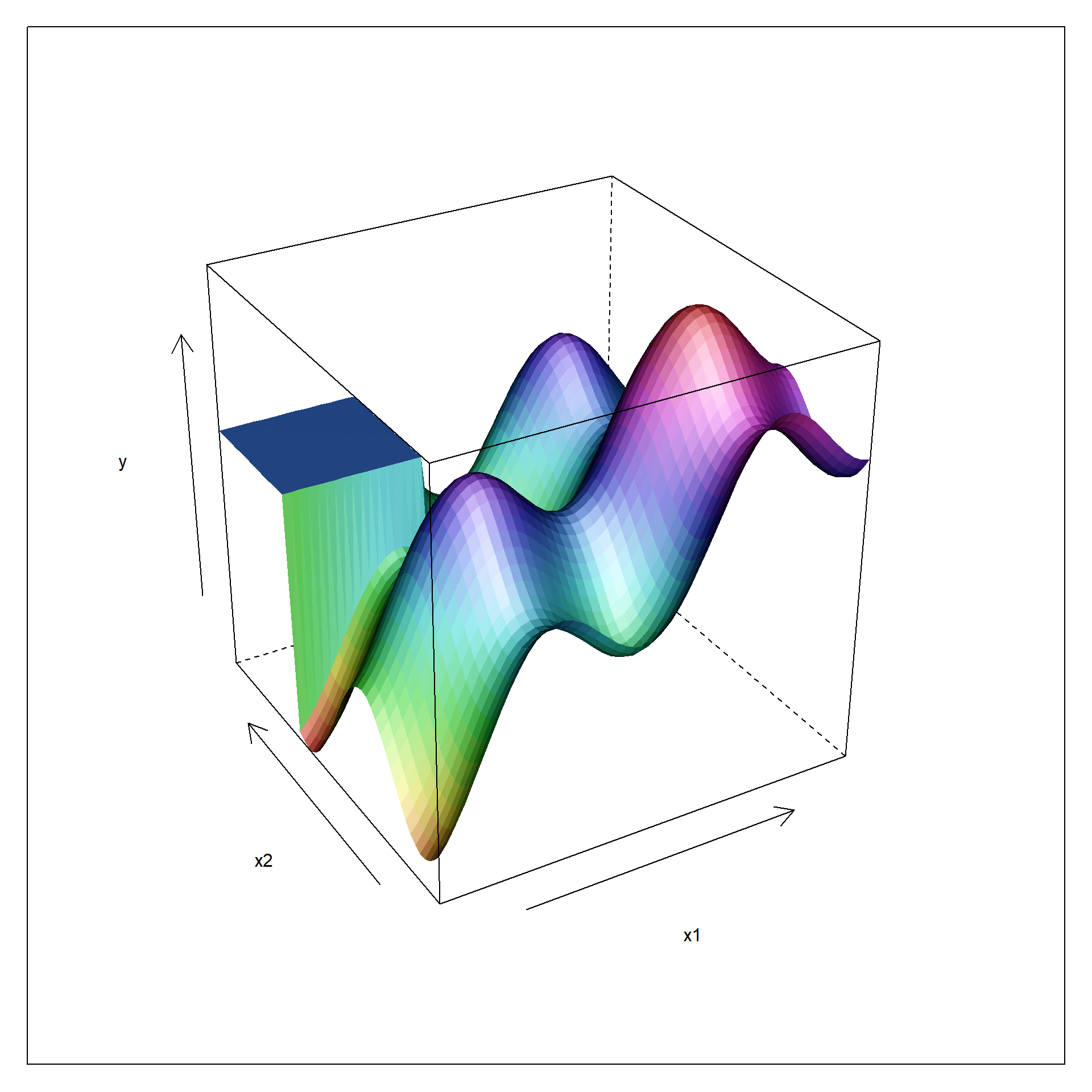
Figure 6.3: Non-linear function with smooth and non-smooth domains in two dimensions

From the figures 6.2 and 6.3 can be concluded that non-convex functions have convex domains which can be locally approximated by convex functions such as linear, bilinear and quadratic DoE surrogates. Consequentially, non-convex functions can be optimized by repeatedly solving locally convex optimization problems without requiring the non-linear function g(x₁,x₂,…x_i) to be known analytically.

6.2 Relaxation and sequential optimization

DoE surrogate functions - linear, bilinear and quadratic parametric functions - are convex and can be used to locally probe the landscape of any smooth non-convex function. The individual steps of this approach can be outlined as follows

1. Create an experimental design in a local domain X rendering all linear effects (linear gradients) and some higher order effects estimable with the latter terms providing information about the non-linearity (curvature) of the local domain.
2. Depending on the outcome - linear or non-linear topology - follow either path of action
   • Linear topology: Ascend (or descend depending on objectives) along the gradient by relaxing the local domain in discrete step thereby creating a sequence of promising conditions in term of the optimization goal. Realize these conditions in the laboratory and proceed relaxing as long as there is improvement.
   • Non-linear topology: Augment the design to render all second order effects estimable. Realize the augmentation trials in the lab, check for local extrema and, if possible, ascend (descend) by relaxing the local domain. Realize the relaxation trials in the lab and proceed as long as there is progress.
3. Use the best relaxation trial from the above sequence as a reference point for an new designs and start repeating the above optimization sequence.

This three step procedure will rapidly and with minimal number of experiments approach the next local extremum. The ideas just described will be illustrated by sequentially optimizing the non-linear function depicted in figure 6.4 as both wireframe and contour plot.

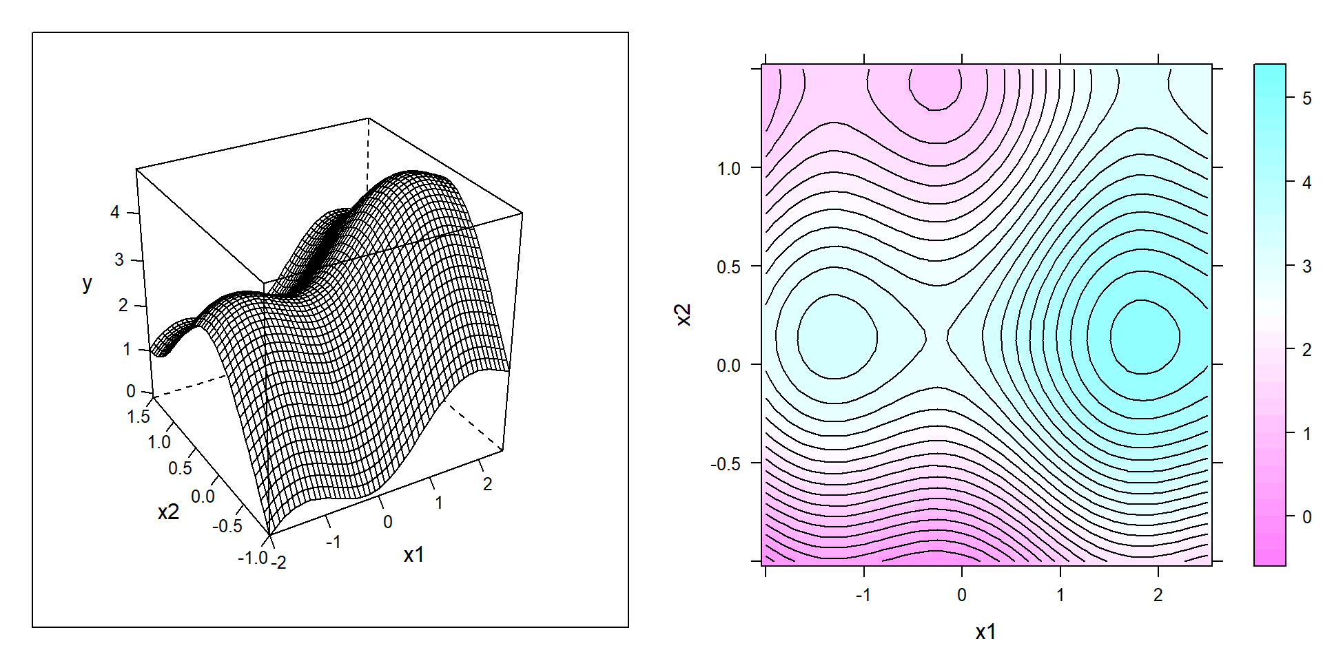
Figure 6.4: Wireframe (left panel) and contour (right panel) plot of a non-convex example function to be “empirically” maximized in the depicted domain x₁,x₂.

Figure 6.4 discerns three local extrema in the domain of interest, that is a marked sattle point between the global maximum in the east and a local maximum in the west. Suppose the aim is finding conditions \(x_{1}^*,x_{2}^*\) maximizing the response y and further suppose that the project locally starts in the south of the domain as depicted by the solid rectangle in figure 6.5.

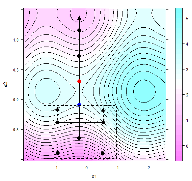
Figure 6.5: Steepest ascend derived from the local topology marked by the solid rectangle in the south. The first relaxation step with the respective relaxation trial marked blue is indicated by the dashed rectangle. The best relaxation trial is labelled red

As a reasonable start design⁴⁶, a full factorial 2x2 design plus center point was created, see the solid rectangle in the south of figure 6.5. Almost certainly the regression model \(y=a_{0}+a_{1}\cdot x_{1}+a_{1}\cdot x_{2} + \epsilon\) will miss the small non-linearities<\(\epsilon\) and will report the OLS solution a₁=0 and a₂>>0 thereby suggesting to ascend to the north of x₂. This process called hypercubical relaxation can be made in silico by solving a constrained optimization problem in k=1,2,3…N discrete steps thus generating a sequence of relaxation trials, \(X_{1}^*,X_{2}^*,...X_{N}^*\). With stepsize \(\Delta X =\Delta x_{1}, \Delta x_{2}\), the lower and upper bounds \(LB=[min(x_{1}),min(x_{2})]\) and \(UB=[max(x_{1}),max(x_{2})]\), respectively, the k relaxation steps can be formulated as a constrained optimization problem \[\large { \max_{X} } \Big (a_{0} + a_{1}\cdot x_{1} + a_{2} \cdot x_{2} \Big ) \] \[subject \ to \] \[ LB-k \cdot \Delta X \leq X \leq UB+k \cdot \Delta X\] Setting k=1,2,3,4 in figure 6.5 will generate a sequence of four relaxation trials in the direction of and traversing the sattle point from which the results start dropping again.
In order to make further progress, a second factorial around the best relaxation trial is set up. This time, the non-linear topology underlying the second design will render the interaction term significant, and the design will therefore be augmented by star points with the resulting CC design shown in figure 6.6.

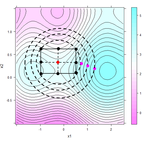
Figure 6.6: Ridge trace relaxation approaching the local optimum (see text for more explanations)

The local response surface model will indicate an ascending ridge stretching to the east in figure 6.6. Again, relaxation trials can be generated using hypercubical relaxation as described above or, alternatively, hyperspherical relaxation can be used to further exploit the local topology. Rather than relaxing box constraints, hyperspherical relaxation works by relaxing a hypersphere in discrete step. With R denoting the radius of the sphere to be relaxed and stepsize \(\Delta r\), the relaxation process can be written concisely \[\large { \max_{X} } \Big (a_{0} + a_{1}\cdot x_{1} + a_{2} \cdot x_{2} + a_{12}\cdot x_{1}\cdot x_{2} + a_{11}\cdot x_{1}^2 + a_{22}\cdot x_{2}^2 \Big ) \] \[ subject \ to \] \[ \sum_{i=1}^2 x^2_{i} \leq (R + k \cdot\Delta r)^2\]
Optimization with hyperspherical constraints is also known in the literature as ridge trace analysis and can be done with the R function steepest() in the package rsm. Usually the results from hypercubical and hyperspherical relaxation are similar with the former being located at the vertices of the domain and the latter more centered.
All concepts discussed so far are put together in the following R-code, namely the following four parts

1. The first code segement #1 creates a response surface with an ascending ridge stretching South-West from the model y = 90 - 8x₁ - 40x₁² - 8x₂ - 80x₂² + 80x₁x₂ + N(0,2).
2. Then the ridge trace of steepest ascend (= set of hyperspherical relaxation trials) is calculated with the function steepest() from the package rsm.
3. Part #3 uses the convex optimizer solnp() from the R-package Rsolnp for creating (here) 20 hypercubical relaxation trials with a step size of (here) 2.5% of the initial X-space. The function solnp() can be extended by any smooth equality and inequality constraints if nescessary. The package can also be used for optimizing non-convex functions by randomly restarting the optimizer at different locations in X so as to increase the chance of finding the global optimum.
4. Finally, the hypercubical and hyperspherical traces are plotted along with the contour lines of the model in figure 6.7.

rm(list=ls())
library(lattice)
library(rsm)
library(pals)
set.seed(123)
############ 1: create a simple ascending ridge in x1,x2 
########################################################
x.grid <- expand.grid(x1= seq(0,1,length=10),
                  x2= seq(0,1,length=10)  )
x.grid$y <- 90  - 8*x.grid$x1 - 40*x.grid$x1^2 - 
            8*x.grid$x2 - 80*x.grid$x2^2 + 
                  80*x.grid$x1*x.grid$x2 + 
            rnorm(nrow(x.grid),0,2)
res.lm <- lm(y ~ x1 +x2 + I(x1^2) + I(x2^2) + x1:x2, data=x.grid)

########## 2: rsm modeling + ridge trace analysis with rsm()
########################################################
x.coded  <- coded.data(x.grid, x1.c~(x1-0.5)/0.25,
                       x2.c ~ (x2-0.5)/0.25)
res.rsm  <- rsm(y ~ SO(x1.c, x2.c ),   data=x.coded)
ridge <- steepest(res.rsm, dist = seq(0,3,0.1), 
          descent=FALSE) #descent=F: max

## Path of steepest ascent from ridge analysis:

head(ridge)

##   dist   x1.c   x2.c |      x1      x2 |   yhat
## 1  0.0  0.000  0.000 | 0.50000 0.50000 | 72.153
## 2  0.1 -0.021 -0.098 | 0.49475 0.47550 | 73.321
## 3  0.2 -0.050 -0.194 | 0.48750 0.45150 | 74.415
## 4  0.3 -0.088 -0.287 | 0.47800 0.42825 | 75.442
## 5  0.4 -0.134 -0.377 | 0.46650 0.40575 | 76.411
## 6  0.5 -0.187 -0.464 | 0.45325 0.38400 | 77.332

############################ 3: hypercubical relaxation 
############################ using Rsolnp

library(Rsolnp)

x.var    <- c("x1","x2")
y.var    <-  "y"
x.mean   <- sapply(x.grid[,x.var],mean,na.rm=T)
x.lb     <-  sapply(x.grid[,x.var],min,na.rm=T) # LB,UB
x.ub     <-  sapply(x.grid[,x.var],max,na.rm=T)
delta    <- (x.ub-x.lb)/40 # stepsize 2.5% of X

df.collect  <- NULL 

objective   =function(x) {      
  xx               <- data.frame(rbind(x))
  colnames(xx)     <- x.var 
  return( -predict(res.lm,xx)  ) # max(x) = min(-x)   
}

for (i in (1:20))   {
  
  xx.lb <- c(0.5,0.5) - i*delta
  xx.ub <- c(0.5,0.5) + i*delta
  
  res.nlp  <- solnp(fun=objective , LB=xx.lb,UB=xx.ub,
                pars=x.mean, control=list(trace=0))
  
  solution           <- rbind(res.nlp$pars)
  colnames(solution) <- x.var
  df.collect         <- rbind(df.collect, data.frame(relax.step=i,
                        y.at.solution = -objective(solution) , 
                        rbind(solution) )  )
}
rownames(df.collect)  <- NULL
head(df.collect)

##   relax.step y.at.solution        x1    x2
## 1          1      73.51149 0.4750001 0.475
## 2          2      74.82308 0.4500000 0.450
## 3          3      76.08742 0.4250001 0.425
## 4          4      77.30450 0.4000001 0.400
## 5          5      78.47434 0.3750001 0.375
## 6          6      79.59693 0.3500001 0.350

# 4: plot hyperspherical + hypercubical trace together
# on 2D contour plot with 3 constraints superimposed

x.pred <- expand.grid(x1= seq(0,1,length=50),
                       x2= seq(0,1,length=50)  )
x.pred$y <- predict(res.lm,x.pred)
p  <- contourplot(y ~ x1*x2, data=x.pred, cuts=50, 
                  labels=F,pretty=T,region=T)
update(p, panel = function(...){
  panel.contourplot(...)
  panel.xyplot(0.5,0.5, pch=16,col="black", cex=1)
  panel.abline(v=0.5,h=0.5, col="black", lty=2)
  panel.xyplot(df.collect[,3],df.collect[,4] , 
               col="blue", pch=16)
  panel.xyplot(ridge[-1,5],ridge[-1,6], col="red", pch=16)
  panel.lines(ridge[-1,5],ridge[-1,6], col="red")
  panel.lines(df.collect[,3],df.collect[,4] , col="blue")
  panel.xyplot(0.5,0.5, pch=1,col="red", cex=4.5)
  panel.xyplot(0.5,0.5, pch=1,col="red", cex=23)
  panel.xyplot(0.5,0.5, pch=1,col="red", cex=39)
  panel.lines(c(0.4,0.4,0.6,0.6,0.4), 
              c(0.4,0.6,0.6,0.4,0.4) , col="blue")
  panel.lines(c(0.35,0.35,0.65,0.65,0.35), 
              c(0.35,0.65,0.65,0.35,0.35) , col="blue")
  panel.lines(c(0.225,0.225,0.775,0.775,0.225), 
              c(0.225,0.775,0.775,0.225,0.225) , col="blue")
})

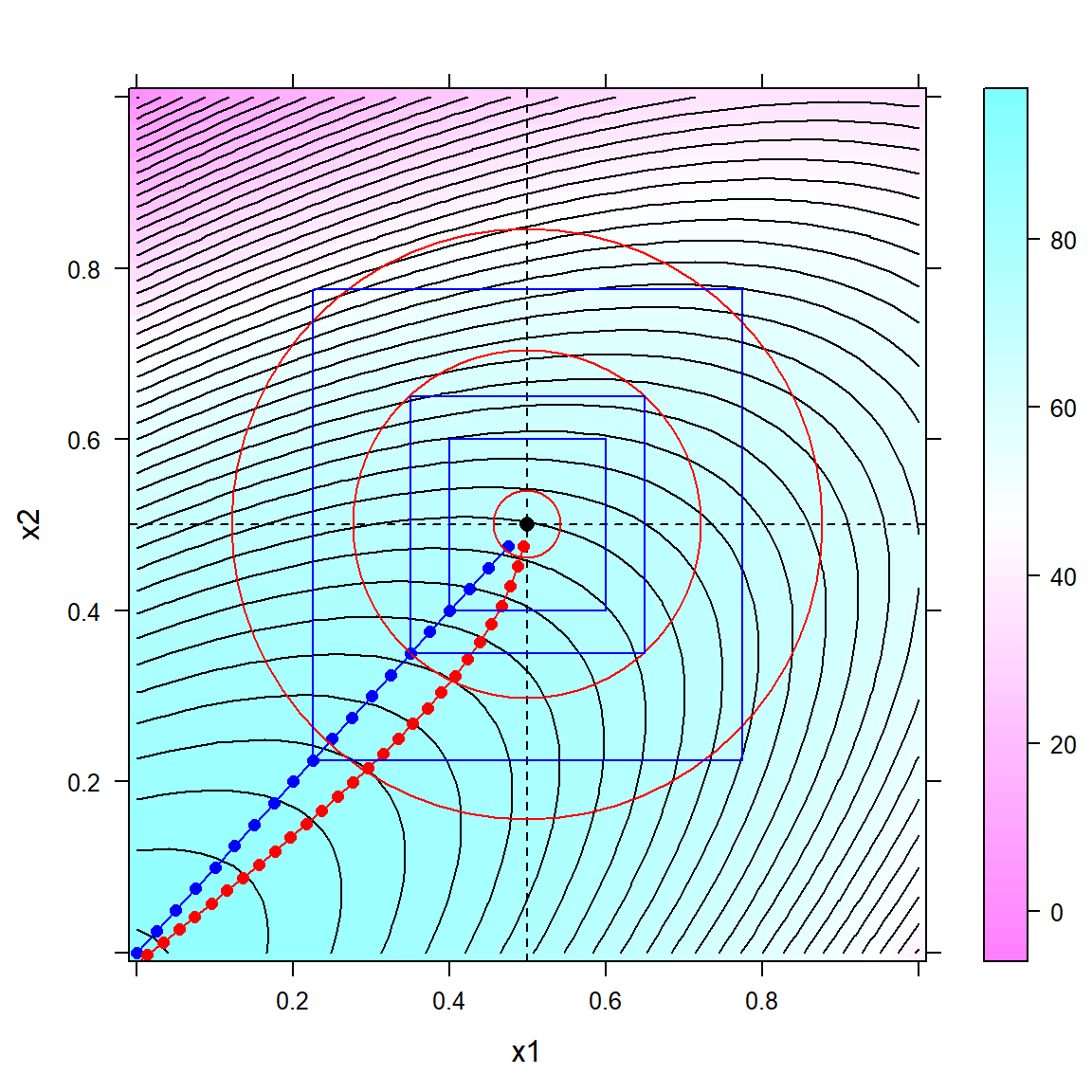
Figure 6.7: Hyperspherical (red) and hypercubical (blue) relaxation traces on an ascending ridge with three hypercubical and hyperspherical constraints superimposed

As revealed in figure 6.7, the ridge trace (in red) is always perpendicular on the curved contour lines of the model and becomes thus curved, different from the straigth line (in blue) of the hypercubical relaxation trace. Generally, the difference between hypercubical and hyperspherical relaxation is often small with the former considered more extreme and the latter more cautious. However, choosing an appropriate stepsize is often more important than choosing the relaxation method, as the stepsize directly affects the degree of extrapolation into an unknown domain. Here, the following rules of thumb apply

1. If the model to be relaxed is linear, bold steps, say \(\Delta=20 \ or \ 30\%\) (or even larger), can be taken after having checked the feasibility of the stepsize with the scientists and technicians.
2. If the model is non-linear (bilinear or quadratic), stepsizes should be choosen smaller (say 1, 2… i% of the initial design space) due to detrimental edge effects of higher order polynomials.

The optimization method just described is in essence a sequential quadratic programming method: The unknown and potentially non-convex objective function is approximated locally by a linear polynom and, if needed, updated by higher order terms and subsequentially relaxed as long as there is progress in terms of the optimization goals. This process comes to a stop when the next local optimum is reached. Global optimality can only be checked by restarting the process just described at a different location in the domain and see whether the solution will converge to a better solution. In empirical optimization projects local optimality in the strict sense is often not nescessary and practical optimality will be sufficient. Relaxation trials meeting the requirements are, to be sure, mathematically not optimal but of practical optimality. Unfortunately, the opposite is also true: Local optima with vanishing first derivatives may not meet the practical optimization goals. When a local optimum misses the practical requirements, it is best to look for new degrees of freedom as new levers to further optimize the system.

6.3 Constrained optimization

So far one objective function was optimized subject to box constraints with the latter being subsequently relaxed in discrete steps as an effective way of multidimensional hill-climbing.
However, optimization has more to offer than just optimizing one objective function subject to box constraints. It can be used to study more complex multidimensional problems hard to oversee otherwise.
The following mixture example is taken from (John A. Cornell 1990), p. 80, and aims at demonstrating the use of constrained optimization for analysing the cost and taste structure of a fruit punch. The design consists of 10 different mixtures and is depicted on the right panel in figure 6.8. The taste of each mixture as the response is scored by three different test persons thus making a total of 30 runs. The data can be analyzed easily using functionalities from the package mixexp (see chapter 5 for more details)., see figure 6.8 for a response surface plot and the modeling details in the R output. Lack of fit⁴⁷, p_lof=0.04, is hardly significant, and the model can be asssumed to unbiasedly describe the data within replication error.

rm(list=ls())
library(Ternary)
library(mixexp)

melon  <- scan(text="1  1   1   0.5 0.5 0.5 0   0   0   0   0   0
              0 0   0   0.5 0.5 0.5 0.33    0.33    0.33
              0.72  0.72    0.72    0.14    0.14    0.14    0.14    0.14    0.14")
pine  <- scan(text="0   0   0   0.5 0.5 0.5 1   1   1   0.5 0.5
                    0.5 0   0   0   0   0   0   0.33    0.33    0.33    0.14
                    0.14    0.14    0.57    0.57    0.57    0.29    0.29    0.29")
orange <- scan(text="0  0   0   0   0   0   0   0   0   0.5 0.5 0.5 1
                    1   1   0.5 0.5 0.5 0.33    0.33    0.33    0.14
                    0.14    0.14    0.29    0.29    0.29    0.57    0.57    0.57")
taste <- scan(text="4.8 4.3 4.7 6.1 6.3 5.8 6.3 6.5 6.2
                    6.1 6.2 6.2 7.4 6.9 7   5.9 6.1 6.5 6.4 6   5.8
                    6.6 5.4 5.8 5.6 5.7 5   6.4 5.2 6.4")

x <- data.frame(melon,pine,orange,taste)

res <- MixModel(x, "taste",
      mixcomps = c("melon", "pine", "orange"), model = 2) 

##      
##              coefficients   Std.err    t.value         Prob
## melon            4.773348 0.2383417 20.0273285 2.220446e-16
## pine             6.266015 0.2473754 25.3299816 0.000000e+00
## orange           7.107707 0.2473754 28.7324717 0.000000e+00
## pine:melon       2.155899 1.1380880  1.8943163 7.029560e-02
## orange:melon     1.105927 1.1380880  0.9717414 3.408717e-01
## pine:orange     -3.529823 1.0195672 -3.4620799 2.023323e-03
##      
## Residual standard error:  0.4351875  on  24 degrees of freedom 
## Corrected Multiple R-squared:  0.6714546

   # reduced cubic

a <- summary(rsm::rsm(taste~ FO(melon,orange) + TWI(melon,orange)
          + PQ(melon,orange), data=x))
a$lof # p.lof=eport lof : p.lof=0.042

## Analysis of Variance Table
## 
## Response: taste
##                    Df Sum Sq Mean Sq F value    Pr(>F)    
## FO(melon, orange)   2 6.1983 3.09915 16.3765 3.271e-05 ***
## TWI(melon, orange)  1 0.1531 0.15307  0.8089  0.377393    
## PQ(melon, orange)   2 2.9414 1.47071  7.7715  0.002499 ** 
## Residuals          24 4.5419 0.18924                      
## Lack of fit         4 1.7152 0.42880  3.0340  0.041640 *  
## Pure error         20 2.8267 0.14133                      
## ---
## Signif. codes:  0 '***' 0.001 '**' 0.01 '*' 0.05 '.' 0.1 ' ' 1

par(mfrow=c(1,2))
plot(predict(res), rstudent(res),
     xlab=expression( paste("predicted response ", hat(y)) )    ,
     ylab="studentized residuals",type="n",
     main=expression(paste("(",frac(paste("y - ",
          hat(y)),sigma), ") ~ ", hat(y)   )) )
colcol <- rep("black",nrow(x))
colcol[duplicated(x[,1:3])]  <- "red"
text(predict(res), rstudent(res),
     col=colcol, label=(1:nrow(x)))
abline(h=c(-2,0,2),lty=c(2,1,2))
grid()

TernaryPlot(atip="melon", btip="pineapple", axis.cex=1.2,lab.cex = 1.3,isometric=F,
            ctip="orange",axis.labels=seq(0,1,0.1))
FunctionToContour <- function (a, b, c) {
  xx <- data.frame(a,b,c)
  colnames(xx) <- c("melon", "pine", "orange")
  return(predict(res,xx))
  }
values            <- TernaryPointValues(FunctionToContour,
                     resolution=24)
ColourTernary(values)
TernaryContour(FunctionToContour, resolution=36)
AddToTernary(points, x[,1:3],pch=16,col="red",cex=1.2)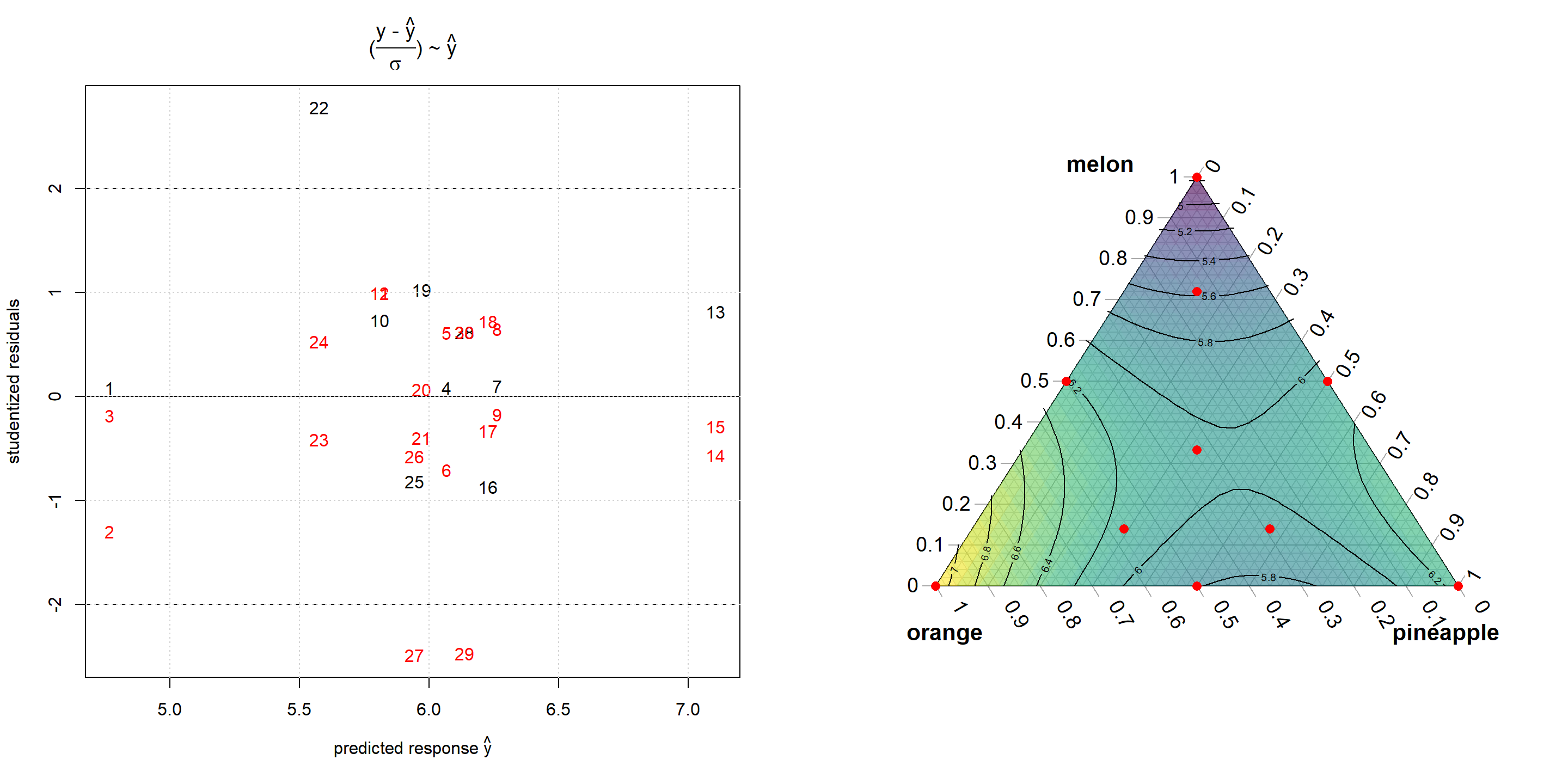

Figure 6.8: Residual analysis (left panel) and contour plot (right panel) from Cornells fruit punch data after being modelled with a quadratic Scheffe model

According to the modeling results, pure orange juice scores best followed by pineapple and watermelon. Pineapple and orange juice reveal an antagonistic interaction rendering binary pineapple orange mixtures less tasty. These conclusions will be further detailed by taking the cost function of the three components into account and setting up a conditional optimization problem. With \(c_{i=1,2,3}=1,2,3\) denoting the cost of the three components \(x_{i}, i=1,2,3\) (melon, pineapple, orange), the conditional optimization problem becomes

\[ \min_{X} \sum_{i=1}^3 (c_{i} \cdot x_{i}) \] \[ subject \ to \] \[ \sum_{i}x_{i}=1 \] \[ taste.LB_{k} \leq taste=f(x_{i}) \leq 10 \]

The following R-code is an implementation of this optimization problem with taste.LB_k being varied in the range of 5.5-7.1. Results are listed in table 6.1, and the optimal results are traced in figure 6.9.

library(Rsolnp)

x.var    <- c("melon", "pine", "orange")
y.var    <-  "taste"
x.mean   <- sapply(x[,x.var],mean,na.rm=T)
x.lb     <-  sapply(x[,x.var],min,na.rm=T) # LB,UB
x.ub     <-  sapply(x[,x.var],max,na.rm=T)
delta    <-  seq(5.5,7.1,0.2) # sequence of lower bounds for taste

df.collect  <- NULL

taste   = function(x) {
  xx               <- data.frame(rbind(x))
  colnames(xx)     <- x.var
  return( predict(res,xx)  ) # max(x) = min(-x)
}

cost = function(x) {
  return(x[1]+ 2*x[2]+ 3*x[3] )
}


for (i in (1:length(delta)) )   {

  res.nlp     <- solnp(fun=cost , LB=x.lb,UB=x.ub,
                       pars=x.mean, eqfun=function(x) {sum(x)},eqB=1,
                      ineqfun=taste, ineqLB=delta[i],
                      ineqUB=10,control=list(trace=0))
  solution     <- (res.nlp$pars)
  df.collect   <- rbind(df.collect, data.frame(step=i,
                           cost.opt = round(cost(solution),3),
                           taste.LB=delta[i],
                           round(rbind(solution),3),
                           taste.opt=round(taste(solution),3),
                           RC=res.nlp$convergence )  )
}
rownames(df.collect)  <- NULL

knitr::kable(
  df.collect, booktabs = TRUE,row.names=F,
  caption = 'Results from taste-constrained cost
  minimization of the fruit juice model')

Table 6.1: Results from taste-constrained cost minimization of the fruit juice model

step	cost.opt	taste.LB	melon	pine	orange	taste.opt	RC
1	1.229	5.5	0.771	0.229	0.000	5.5	0
2	1.308	5.7	0.692	0.308	0.000	5.7	0
3	1.402	5.9	0.598	0.402	0.000	5.9	0
4	1.895	6.1	0.553	0.000	0.447	6.1	0
5	2.064	6.3	0.468	0.000	0.532	6.3	0
6	2.250	6.5	0.375	0.000	0.625	6.5	0
7	2.457	6.7	0.271	0.000	0.729	6.7	0
8	2.697	6.9	0.151	0.000	0.849	6.9	0
9	2.992	7.1	0.004	0.000	0.996	7.1	0

TernaryPlot(atip="melon", btip="pineapple", ctip="orange",axis.cex=0.7,lab.cex = 0.8,
            axis.labels=seq(0,1,0.1))
AddToTernary(points, df.collect[,4:6],pch=16,col="red", cex=1)
TernaryArrows(df.collect[1,4:6],   df.collect[3,4:6],
              col="red",lty=1,lwd=2,length=0.1)
TernaryArrows(df.collect[3,4:6],   df.collect[4,4:6], 
              col="red",lty=1,lwd=2,length=0.1)
TernaryArrows(df.collect[4,4:6],   df.collect[9,4:6],  
              col="red",lty=1,lwd=2,length=0.1)
FunctionToContour <- function (a, b, c) { a + 2*b + 3*c  }
values            <- TernaryPointValues(FunctionToContour, resolution=24)
ColourTernary(values)
TernaryContour(FunctionToContour, resolution=36)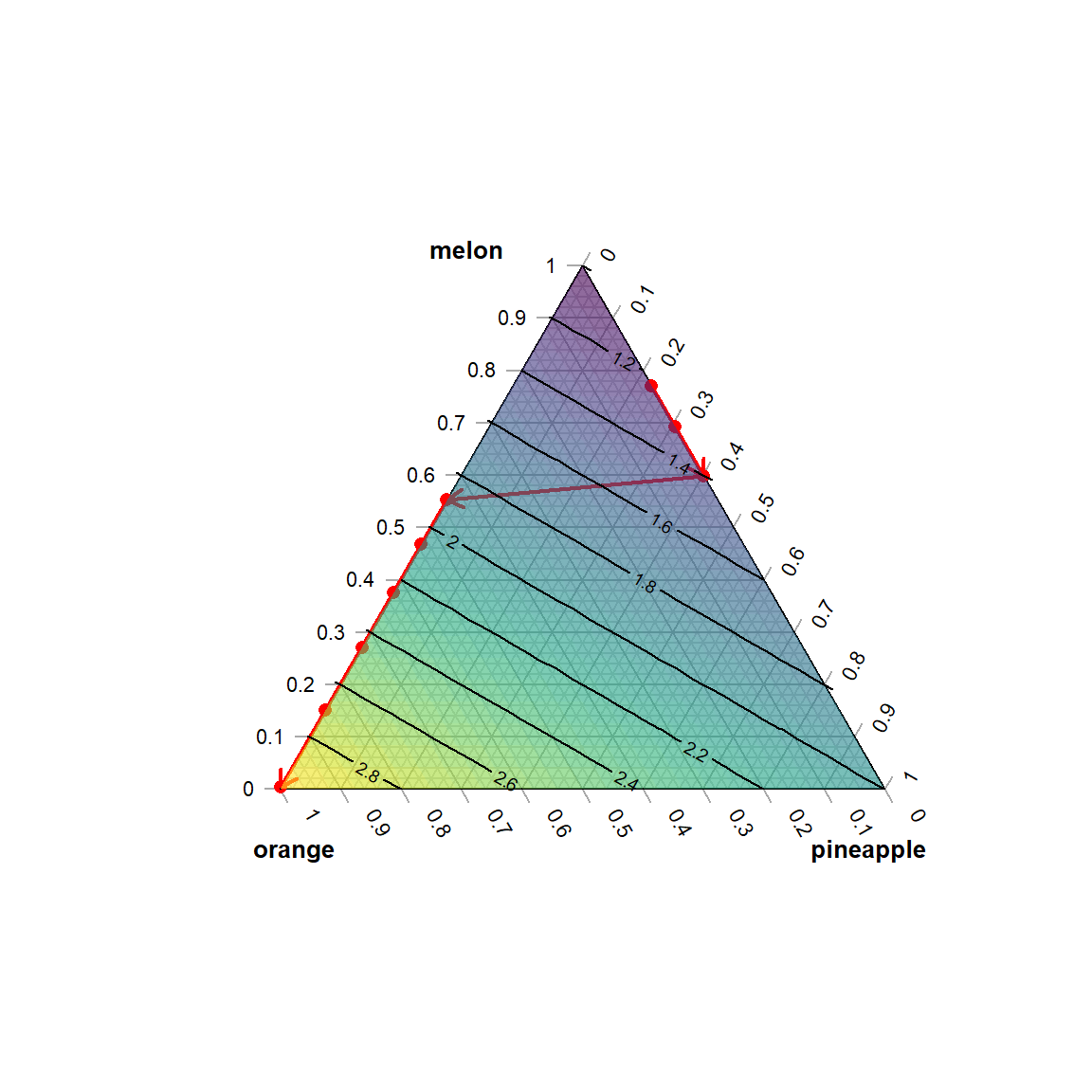

Figure 6.9: Contour plot at minimal costs as a function of increasing taste with direction of increase indicated by arrows

The optimal trace plotted in figure 6.9 describes the cheapest mixtures with an expected taste of at least taste.LB_k. The mixtures found are entirely binary in nature: For taste.LB<5.9 pineapple-melon mixtures are cheapest and better tasting candidates are entirely made of orange-watermelon with watermelon subsequently replaced by orange in the further optimization course. In all nine solutions the lower bound condition is active, i.e. at the optimal solution the equality \(taste.LB_{k} = taste.LB_{k}^*\) holds, and taste actively constrains the cost function. Put differently: By relaxing the lower taste constraint, that is here, lowering taste.LB, the objective function will further decrease.

6.4 Multiresponse optimization

In real-world projects, there are often many responses, formally y_j=g_j(x_i), and scientists tend to state their project goals as a multiresponse task such as max(y₁,y₂,…y_k), min(y_k+1,y_k+2,…y_K). In a strict mathematical sense, such statements are not proper optimization statements because a solution \(X_{i}^*\) maximizing \(y_{1}=f(X_{i}^*)\) does not nescessarily minimize y₂ at the same location \(X_{i}^*\). However, the above multiresponse optimization statements are acceptable by convention and can be tweaked into proper optimization problems.
Prior to implementing a multiresponse optimization problem, the joint correlation structure of the raw data y₁,y₂,…y_k should be analyses thoroughly. For instance, if y₁ and y₂ turn out to be negatively correlated and the aim is joint maximization of both responses, any attempt to maximize both y₁ and y₂ over X will fail. Whatever the optimizer does for maximizing y₁ will inevitably minimize y₂, and including such conflicting responses in a joint optimization problem is not a good advice. Conflicts of aims have there cause in the underlying degrees of freedom (DF) (the X-factors). When there are conflicts of aims it is usually better to stop working with the present DFs and to look for other, more suitable DFs. The ideal DF in a multiresponse optimization problem is a factor affecting one response while leaving the other responses unaffected.
However, if the outcome of exploratory data analysis, here analysis of the joint distribution of y₁ and y₂, is similar to figure 6.10, the “outliers” labelled red should be replicated, as they may indicate conditions in accordance with the joint maximization goal. In this case, rather than trying to optimize y_1,2=f_1,2(x_i), the X-conditions of the “outliers” should be taken as a reference (center) point for a new design which may now lead to a potentially feasible optimization problem.

rm(list=ls())
set.seed(123334)
x <- seq(1,10,length=10)
y <- -1*x + rnorm(length(x),0,1)
plot(x,y,type="p",axes=F,pch=16,
xlab=expression(plain(y) [1]),
ylab=expression(plain(y) [2]))
abline(lm(y~x)$coef)
points(c(10,9,9.5),c(-2,-2.5,-3),col="red",pch=16)
box()

Figure 6.10: Joint distribution \(y_{1},y_{2}\) with promising “outliers” labelled red given goal \(\max_{X}[y_{1}=f_{1}(X),y_{2}=f_{2}(X)]\).

Now, assume for the time being, that conflicting responses are not presents, and the responses are sufficiently independent to render the optimization problem feasible.
One way of optimizing a multiresponse system is similar to the technique described in the previous section and boils down to rewritting the multipresponse problem into a constrained optimization problem with the constraint boundaries made flexible. For instance, the simple statement max(y₁,y₂,y₃) could be rewritten into \[\max_{X} (y_{1}=f_{1}(X)) \] \[ subject \ to \] \[ y_{2}=f_{2}(X) > LB_{2} \] \[y_{3}=f_{3}(X) > LB_{3}\]

By successively increasing LB_i and LB_k, the optimization will be driven to a direction simultaneously maximizing y₁,y₂,y₃ until the solutions become infeasible. When joint minimization is the aim, the problem simply becomes \[\min_{X} (y_{1}=f_{1}(X)) \] \[ subject \ to \] \[ y_{2}=f_{2}(X) < UB_{2} \] \[ y_{3}=f_{3}(X) < UB_{3}\] to the effect that the solution is driven to areas in X-space jointly minimizing y₁,y₂,y₃ When there are many responses to optimize this approach can becomes awkward and a more convenient method is obtained by using convex penalties. The idea is simple and expressed in formula (6.2)

\[\begin{equation} z(x_{1},x_{2},...x_{i}) = \sum_{j=1}^K \Big (\frac {y_{j}- T_{j}} {UB_{j}-LB_{j}} \Big )^2 =\sum_{j=1}^K \Big (\frac {f_{j}(x_{1},x_{2},...x_{i})- T_{j}} {UB_{j}-LB_{j}} \Big )^2 \tag{6.2} \end{equation}\]

with T_j being the desired target values for response y_j and LB_j,UB_j the corresponding lower and upper acceptance boundaries. Depending on the optimization problem, the penalty,(6.2), can be made half-sided with the right sided penalty z()⁺ given by

\[z(x_{1},x_{2},...x_{i})^+ = \sum_{j=1}^K max \Big (0,\frac {f_{j}(x_{1},x_{2},...x_{i})- T_{j}} {UB_{j}-LB_{j}} \Big)^2\] and the corresponding left sided version z()^- \[z(x_{1},x_{2},...x_{i})^- =\sum_{j=1}^K min \Big (0,\frac {f_{j}(x_{1},x_{2},...x_{i})- T_{j}} {UB_{j}-LB_{j}} \Big)^2\] Figure 6.11 shows two symmetric penalty terms with narrow and wide acceptance ranges and two half-sided penalties, z()^+,-. Note how the width of the acceptance range affects the shape and the penalty incured by deviating from the target.

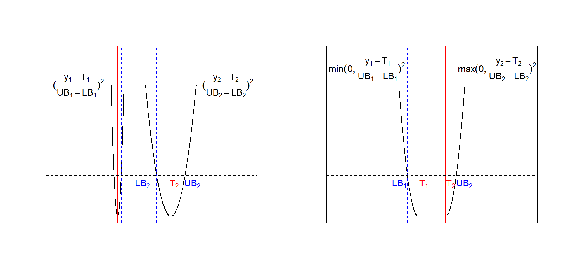
Figure 6.11: Convex penalty functions with narrow and wide acceptance range UB_i-LB_i (left panel) and half-sided convex penalties (right panel)

With the objective, formula (6.2), the multiresponse optimization simply becomes \[ \min_{X} z(x_{1,},x_{2},...x_{i})\] Sums of convex functions are again convex, and \(z(x_{1,},x_{2},...x_{i})\) can therefore be optimized with any convex solver. Here we demonstrate the use of the quasi-global solver gosolnp() from the package Rsolnp for optimizing three scenarios of the fruit punch example from above⁴⁸, namely

1. Scenario #1: T_cost=1.2 +/- 0.001 ; T_taste=7 +/- 0.1
2. Scenario #2: T_cost=1.2 +/- 0.2 ; T_taste=7 +/- 0.0001
3. Scenario #3: T_cost=2 +/- 1 ; T_taste=2 +/- 1

The scenarios differ by putting different weight to the individual terms of the objective function. In scenario #1, e.g., much weight is put on the cost target, cost=1.2 and, as a consequence, the desired target is realized in the solution (see R output from scenario #1).

rm(list=ls())

melon  <- scan(text="1  1   1   0.5 0.5 0.5 0   0   0   0   0   0
              0 0   0   0.5 0.5 0.5 0.33    0.33    0.33
              0.72  0.72    0.72    0.14    0.14    0.14    0.14    0.14    0.14")
pine  <- scan(text="0   0   0   0.5 0.5 0.5 1   1   1   0.5 0.5
                    0.5 0   0   0   0   0   0   0.33    0.33    0.33    0.14
                    0.14    0.14    0.57    0.57    0.57    0.29    0.29    0.29")
orange <- scan(text="0  0   0   0   0   0   0   0   0   0.5 0.5 0.5 1
                    1   1   0.5 0.5 0.5 0.33    0.33    0.33    0.14
                    0.14    0.14    0.29    0.29    0.29    0.57    0.57    0.57")
taste <- scan(text="4.8 4.3 4.7 6.1 6.3 5.8 6.3 6.5 6.2
                    6.1 6.2 6.2 7.4 6.9 7   5.9 6.1 6.5 6.4 6   5.8
                    6.6 5.4 5.8 5.6 5.7 5   6.4 5.2 6.4")

x <- data.frame(melon,pine,orange,taste)

x.var    <- c("melon", "pine", "orange")
y.var    <-  "taste"
x.mean   <-  sapply(x[,x.var],mean,na.rm=T)
x.lb     <-  sapply(x[,x.var],min,na.rm=T) # LB,UB
x.ub     <-  sapply(x[,x.var],max,na.rm=T)

res <- lm( taste~ (melon + pine + orange)^2,  data=x)

taste   = function(x) {
  xx               <- data.frame(rbind(x))
  colnames(xx)     <- x.var
  return( as.numeric(predict(res,xx)) )
}

cost = function(x) {
   return(as.numeric(x[1]+ 2*x[2]+ 3*x[3]))
}

penalty <- function(x) {
  sum( ( (c(cost(x),taste(x) ) -t)/(ub-lb) )^2 )
}

######### scenario 1
lb <- c(1.1999 , 6.9) 
# min(cost)(<=>cost=1.2) given taste
# =>  melon=0.8, pine=0.2
t  <- c(1.2 , 7)
ub <- c(1.2001 , 7.1)

system.time(res.nlp <- Rsolnp::gosolnp(fun=penalty , 
                      LB=x.lb,UB=x.ub, par=x.mean,
                      eqfun=function(x) {sum(x)},eqB=1,  n.restarts = 5,
                      n.sim = 10000, rseed=12345,control=list(trace=0)))

##    user  system elapsed 
##   30.13    0.48   31.30

res.nlp$pars

##        melon         pine       orange 
## 7.999958e-01 2.000042e-01 5.638882e-11

cost(res.nlp$pars)

## [1] 1.200004

taste(res.nlp$pars)

## [1] 5.409904

################################# scenario 2
lb <- c(1 , 6.9999) 
# max(taste)(<=>taste=7) given cost; 
# => melon=0.08, orange=0.92,
t  <- c(1.2 , 7)
ub <- c(1.4 , 7.0001)

system.time(res.nlp <- Rsolnp::gosolnp(fun=penalty ,
                      LB=x.lb,UB=x.ub, par=x.mean,
                      eqfun=function(x) {sum(x)},eqB=1,  n.restarts = 5,
                      n.sim = 10000, rseed=12345,control=list(trace=0)))

##    user  system elapsed 
##   30.28    1.09   32.62

res.nlp$pars

##        melon         pine       orange 
## 8.070163e-02 1.263921e-10 9.192984e-01

cost(res.nlp$pars)

## [1] 2.838597

taste(res.nlp$pars)

## [1] 7

################################# scenario 3

lb <- c(1 , 5) 
# max(taste)(<=>taste=7) given cost; 
# => melon=0.33, pine=0.33, orange=0.33,
t  <- c(2 , 6)
ub <- c(3 , 7)

system.time(res.nlp <- Rsolnp::gosolnp(fun=penalty , 
                      LB=x.lb,UB=x.ub, par=x.mean,
                      eqfun=function(x) {sum(x)},eqB=1,  n.restarts = 5,
                      n.sim = 10000, rseed=12345,control=list(trace=0)))

##    user  system elapsed 
##   29.05    0.72   30.47

res.nlp$pars

##     melon      pine    orange 
## 0.3319041 0.3361917 0.3319042

cost(res.nlp$pars)

## [1] 2

taste(res.nlp$pars)

## [1] 6

The conclusion from these optimization scenarios agree with the results from constrained optimization: Tasty mixtures are expensive and are made primarily of (expensive) orange juice with watermelon acting as a cheap filler.
Cheap mixtures are less tasty blends of cheap watermelon with cheap pineapple.
Overall, in the fruit punch example there are no degrees of freedom to simultaneously minimize cost and maximize taste, because the expensive component is also the one required for good taste. An average mixture balancing cost and taste is the centroid point suggested by the third optimization scenario.

6.5 Optimization of derived responses

The previous sections discussed joint and multidimensional optimization problems over a set of measured responses. However, in the physical and chemical sciences optimization problems are often stated in terms of derived responses, these are functions of measured responses, z=f(y₁, y₂, …y_j). For instance, in chemistry, the goal can often be stated as: “Find conditions \(X^*\) maximizing the sum of the main product while minimizing the sum of the by-products”, formally \[ \max_{X} \sum_{j=1}^{N_{1}} mp_{j}(x_{1},x_{2}...x_{i}) \] \[ and \] \[ \min_{X} \sum_{j=1}^{N_{2}} bp_{j}(x_{1},x_{2}...x_{i})\] It is a widespread habit among experimentally working scientists, especially in times of readily available spreadsheet programms, to functionally convert the raw measured responses y_j into derived responses z_k=f_k(y_j) and treat these variables subsequently as if they were measured responses. However, empirical model building and optimization should never be based on derived responses, rather it should always be based on measured responses. There are two good reasons for this advice, namely

1. The measured values y_j are random variables with variances \(\sigma_{j}^2\) as a consequence of \(y_{j}=f_{j}(x_{i}) + \epsilon_{j}; \ \epsilon_{j} \sim N(0,\sigma_{j}^2)\). According to the laws of statistics,⁴⁹ aggregation of several responses into a derived response will inflate the error of the new response. For instance, simply adding responses, \(\sum_{i}y_{i}\), amounts to adding the variance of the individual responses, \(Var(\sum_{j]}y_{j})=\sum_{j} \sigma_{j}^2\) (see⁵⁰ ). Now, the variances of the models \(\hat y_{j}=f_{j}(x_{i})\) are much smaller than Var(y_j)⁵¹, therefore summing \(\hat y_{j}\) is to be prefered over summing \(y_{j}\).
2. When \(y_{j}=f_{j}(x_{i}) + \epsilon_{j}\) is linear in x_i, transformation z=f(y_j) will likely render z non-linear in x_i in this way making empirical building more rather then less complex. It is therefore adviced to do the model building step with the measured responses only and use the parametric surrogates \(\hat y_{j}=g_{j}(x_{i})\) for defining the derived responses \(z(x_{i})=f(g_{j}(x_{i}))\). Irrespective of whether z is convex or non-convex, and it can become non-convex esily, optimizers such as gosolnp() can deal with such non-linearities and find reliable solutions.

The following R-simulation makes the above arguments transparent. First two responses, \(y_{1,2}=f_{1,2}(x_{1},x_{2}) + \epsilon_{1,2}; \ \epsilon_{1,2} \sim N(0,\sigma_{1,2}^2)=1;\ Cov(\epsilon_{1},\epsilon_{2})=0\), are defined with both being linear in x_i. Then a realization of the derived response z(x₁,x₂) is created from the “experimental” values with the transformation \(z=100-\frac{y_{1}}{y_{2}}\). The “true” z, here called Z, with \(Z=100-\frac{f_{1}(x_{1},x_{2})}{f_{2}(x_{1},x_{2})}\) is shown in figure 6.12.

rm(list=ls())
set.seed(123)
x <- expand.grid(x1=seq(0.1,1,length=50), x2=seq(0.1,1,length=50) )
x.var    <- c("x1", "x2")
x.mean   <-  sapply(x[,x.var],mean,na.rm=T)
x.ub     <-  sapply(x[,x.var],max,na.rm=T)
x.lb     <-  sapply(x[,x.var],min,na.rm=T)
x$y1 <- 10  -3*x$x1 + 2*x$x2   + rnorm(nrow(x),0,1)
x$y2 <- 20 +  50*x$x1 - 20*x$x2 + rnorm(nrow(x),0,1)
x$z  <- 100 - (x$y1/x$y2)
sapply(x,range)

##       x1  x2        y1        y2        z
## [1,] 0.1 0.1  5.290225  3.466876 96.14665
## [2,] 1.0 1.0 13.798293 68.373127 99.91605

x$yy <- 100 - (10  -3*x$x1 + 2*x$x2  ) / (20 +  50*x$x1 - 20*x$x2)
lattice::wireframe(yy ~ x1*x2, data=x , scales = list(arrows = F),drape=F,zlab="Z",
                   screen = list(z = 30, x = -60),zlim=c(97.5,100))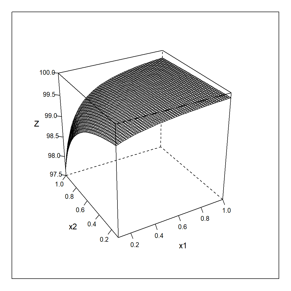

Figure 6.12: Wireframe plot of the “true” derived response \(Z=100 - \frac{f_{1}}{f_{2}}\) as a function of \(x_{1},x_{2}\).

As expected Z is non-linear hyperbolic, and so the realization z=f(x₁,x₂) can be expected non-linear, too. This is in fact the case as the empirical model building step shows, and z needs to be modelled with a quadratic regression model, z=rsm(x_i). However, residual diagnostics shows (not included in the code and left as an excercise) that the model is still biased and does not appropriately describe the data. Figure 6.13 compares the response surface of the unbiased model \(\hat z.derived=100-\frac{\hat y_{1}}{\hat y_{2}}\) with the biased RSM model \(\hat z.rsm \sim x_{1} + x_{2} + x_{1}\cdot x_{2} +x_{1}^2+x_{2}^2\). The relationship \(100-\frac{\hat y_{1}}{\hat y_{2}}\) depicted on the left of figure 6.13 cannot be described unbiasedly by the RSM model, and the quadratic model creates an artificial ridge in an attempt to fit the hyperbolic relationship. As a consequence the “true” maximum at \(x_{1}^*=1; x_{2}^*=0.1\) is missed and an artifical maximum is created at \(x_{1}^*=0.74; x_{2}^*=0.34\).

        res1  <- lm(y1~(x1+x2) ,data=x)
        res2  <- lm(y2~(x1+x2) ,data=x)
summary(res.z <- lm(z~(x1+x2)^2 + I(x1^2)+ I(x2^2),data=x))

## 
## Call:
## lm(formula = z ~ (x1 + x2)^2 + I(x1^2) + I(x2^2), data = x)
## 
## Residuals:
##      Min       1Q   Median       3Q      Max 
## -2.62157 -0.03968 -0.00667  0.04400  0.30168 
## 
## Coefficients:
##             Estimate Std. Error t value Pr(>|t|)    
## (Intercept) 99.46314    0.01556 6392.63   <2e-16 ***
## x1           1.40641    0.04084   34.44   <2e-16 ***
## x2          -0.60462    0.04084  -14.81   <2e-16 ***
## I(x1^2)     -1.24237    0.03326  -37.36   <2e-16 ***
## I(x2^2)     -0.38020    0.03326  -11.43   <2e-16 ***
## x1:x2        1.18976    0.02973   40.02   <2e-16 ***
## ---
## Signif. codes:  0 '***' 0.001 '**' 0.01 '*' 0.05 '.' 0.1 ' ' 1
## 
## Residual standard error: 0.1044 on 2494 degrees of freedom
## Multiple R-squared:  0.8398, Adjusted R-squared:  0.8395 
## F-statistic:  2615 on 5 and 2494 DF,  p-value: < 2.2e-16

x$z.derived   <- (100 - predict(res1,x)/predict(res2,x)  ) 
x$z.rsm       <- predict(res.z,x)

p1  <- lattice::wireframe(z.derived ~ x1*x2, data=x , 
       scales = list(arrows = FALSE,
                                 x=c(cex=1.1),
                                 y=c(cex=1.1),
                                 z=c(cex=1.1)) ,
       drape=F,zlim=c(97.5,100),
       screen = list(z = 30, x = -60), 
       zlab=list(label="z.derived",rot=90),
        xlab=list(label=expression(x [1]),rot=0,cex=1.1),
        ylab=list(label=expression(x [2]), rot=0,cex=1.1) )
p2  <- lattice::wireframe(z.rsm ~ x1*x2, data=x , 
       scales = list(arrows = FALSE,
                                 x=c(cex=1.1),
                                 y=c(cex=1.1),
                                 z=c(cex=1.1)) ,
       drape=F,zlim=c(97.5,100),
       screen = list(z = 30, x = -60), 
       zlab=list(label="z.rsm",rot=90),
       xlab=list(label=expression(x [1]),rot=0,cex=1.1),
        ylab=list(label=expression(x [2]), rot=0,cex=1.1) )
plot(p1,split=c(1,1,2,1),more=T)  # split = c(col,row,ncol,nrow)
plot(p2,split=c(2,1,2,1),more=T)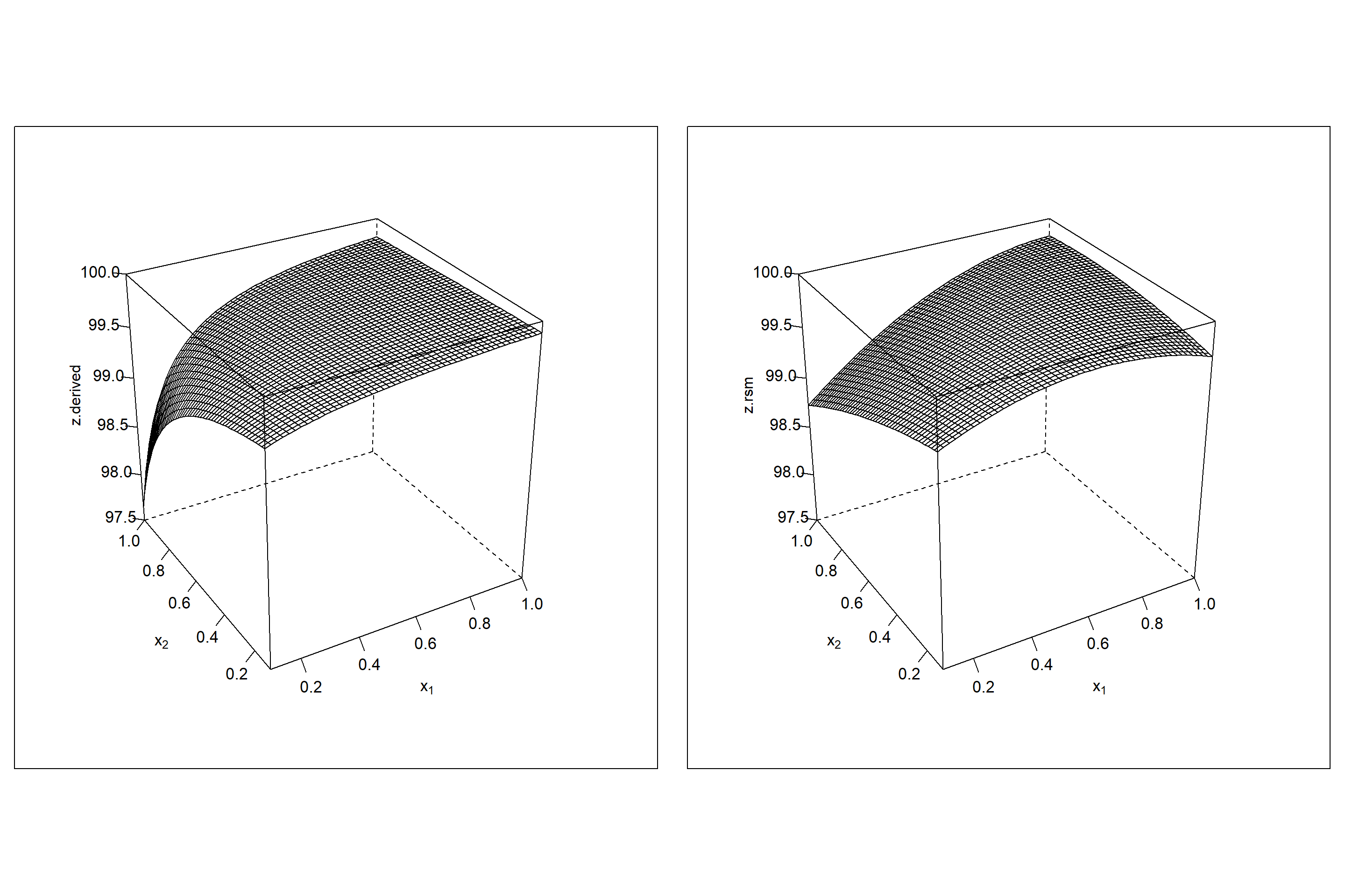  

Figure 6.13: Wireframe plot of \(\hat z.derived=100 - \frac{\hat f_{1}}{\hat f_{2}}\) (left panel) and estimated \(\hat z.rsm=rsm(100 - \frac{y_{1}}{y_{2}})\) (right panel) as a function of \(x_{1},x_{2}\).

##definition objective functions to be maximized

# the function 100 - (y1.hat/y2.hat) (taken negative for max)
obj.y1.y2 <- function(x) {
    xx               <- data.frame(rbind(x))
    colnames(xx)     <- x.var
    return(-(100 - predict(res1,xx)/predict(res2,xx)  ) )  # min
  }

# the function z.hat
obj.z <- function(x) {
  xx               <- data.frame(rbind(x))
  colnames(xx)     <- x.var
  return(- predict(res.z,xx)  )
}

# scenario 1: max(100 - (y1.hat/y2.hat)) ; 
# correct maximum at x1=1;x2=0.1
system.time(res.nlp1 <- Rsolnp::gosolnp(fun=obj.y1.y2 , 
                        LB=x.lb,UB=x.ub, par=x.mean,
                        n.restarts = 1,
                        n.sim = 10000, rseed=12345,
                        control=list(trace=0)))

##    user  system elapsed 
##    9.10    0.12    9.44

round(res.nlp1$pars,3)

##  x1  x2 
## 1.0 0.1

res.nlp1$convergence # 0

## [1] 0

# scenario 2: max(z.hat) ; 
# erroneous maximum at x1=0.739,x2=0.361
system.time(res.nlp2 <- Rsolnp::gosolnp(fun=obj.z, 
                        LB=x.lb,UB=x.ub, par=x.mean,
                        n.restarts = 1,
                        n.sim = 10000, rseed=12345,
                        control=list(trace=0)))

##    user  system elapsed 
##    7.06    0.14    7.44

round(res.nlp2$pars,3)

##    x1    x2 
## 0.739 0.361

res.nlp2$convergence # 0

## [1] 0

The example impressively demonstrated how arithmetics with measured responses can turn a simple model building problem into a hard modeling problem, which cannot be handled anymore with simple polynomial surrogate functions. So, the habit of doing arithmetics with measured responses should better become a habit of bygone times.

Reference

John A. Cornell. 1990. Experiments with Mixtures. 2nd ed. Wiley, New York.

---

44. Projects fail because in the domain X of the optimization problem the constraints are nowhere met. When this happens the optimization problem is called infeasible.↩

45. For an overview of global optimization methods in R see, e.g., (K.M. Mullen 2014)↩

46. A start design must support all linear effects (the gradient) and should at least support some interactions for providing information on 2_nd-order effects in the domain. These requirements naturally suggest full factorial or fractional factorial designs as starting candidates.↩

47. Note that the Lof statistics is obtained by using the function rsm::rsm() on the slack variable model↩

48. n.sim=10000 creates 10000 points in mixture space and evaluates the objective function. The optimizer is then initialized with the X set thus found. The option n.restarts=5 repeats this process five times, so in total 50000 function evaluation were performed to generate “good” local starting values. Strictly, gosolnp() is not necessary for the objective \(z(x_{1,},x_{2},...x_{i})\) (solnp() would be sufficient for z()) but shown here as an example for approaching global optimization problems.↩

49. see (J.G. Kalbfleisch 1985), Vol. I, pp. 182-187.↩

50. the variance of a weighted sum of random variables y_j is given by \(Var(\sum_{j} a_{j}y_{j}) = \sum_{j}a_{j}^2\cdot Var(y_{j}) + 2\sum_{j>i}a_{i}a_{j}\cdot Cov(y_{i},y_{j})\) with \(Var(y_{j})=Var(\epsilon_{j})=\sigma_{j}^2\) and \(Cov(y_{i},y_{j})=Cov(\epsilon_{i},\epsilon_{j})=0\).↩

51. An example might be helpful here: If we take a N-sample from a normal distribution with variance \(\sigma^2\) than each observations has variance \(\sigma^2\). The mean of this sample can be written as the least squares estimate \(a_{0}\) of the linear regression model, \(\hat y=\bar y=a_{0}\), which has variance \(\frac{\sigma^2}{N}\). More generally, for a linear parametric model \(\hat y = f(x_{0}|a_{i})\) at x-location \(x_{0}\) the variance is given by \(Var(\hat y)=[x_{0}^T\cdot(X^T\cdot X)^{-1}\cdot x_{0}]\cdot \sigma^2\). \(Var(\hat y(x_{0}))\) gives a number in the order of magnitude \(\approx \frac{\sigma^2}{N}\), and that explains why the model error is so much smaller than the sampling error. Note again, how the design \(X\) affects the model error by the term \((X^T\cdot X)^{-1}\).↩