4 Design of Experiments (DoE)
This chapter introduces experimental design as an essential part of OLS modeling, Many important design classes will be discussed together with the associated OLS models for analysing these designs. It will be outlined that collinearity, due to a poorly designed matrix X, is the driving force for the methology of experimental design (Design of Experiments, DoE).
4.1 OLS and collinearity
In chapter 3.4.3.4 DoE was loosely defined as the process of minimizing the objective function \(Var(\hat \beta)\) over X, formally \[ \large {\min_{\boldsymbol X}\sigma ^{2} } \large \boldsymbol {(X^{T}X)^{-1}}\] The expression \(Var(\hat \beta)\) is a matrix and must first be converted into a scalar function \(g(X)=f(Var(\hat \beta))\) which can then be optimized as a function of the design X. The optimization problem thus becomes \[\large {\min_{\boldsymbol X}\sigma ^{2} f} \big (\boldsymbol {(X^{T}X)^{-1}}\big )\] with the scalar functional f() belonging to the class of the so called alphabetic functions seeking different kinds of optimality (A-,C-,D-,E-,G-optimality to name but a few)23.
Alphabetic optimality aims at minimizing the uncertainty of the OLS estimates \(\hat \beta\) over the design matrix X or to render the design X maximal robust and informative given the experimental uncertainty \(\sigma^2\).
Now, in order to understand the mechanism of how different designs X can affect the outcome of OLS, let us consider two different designs for identifying the “true” model \(y = 3 + 2 \cdot x_{1} + 5 \cdot x_{2} + \epsilon; \epsilon \sim N(0,1)\)
- An orthogonal 2x2 full factorial design as a triple replicate with Pearson-r, r(x1,x2) = 0
- A collineare design with x1= x2 + N(0,0.5) with Pearson-r, r(x1,x2) = +0.94
Both designs along with the estimated regression planes are depicted in figure 4.1.
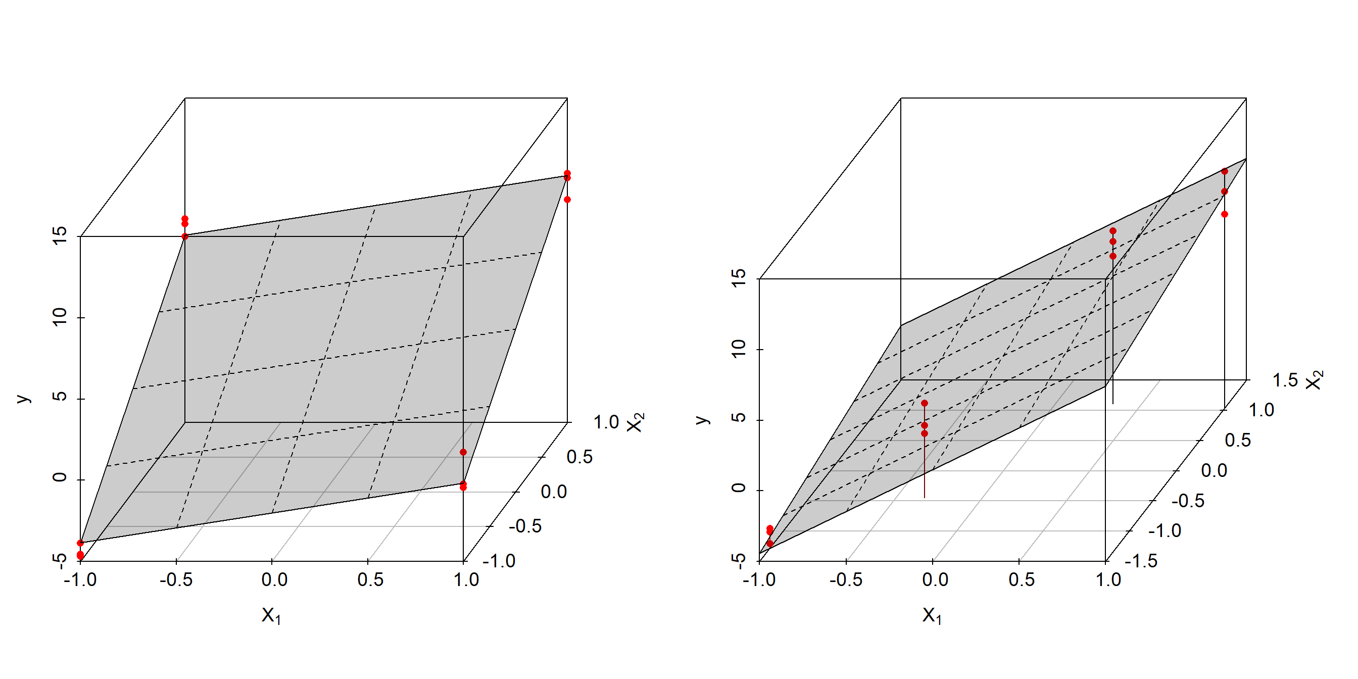
Figure 4.1: Linear OLS model \(y=a_{0} + a_{1} \cdot x_{1} + a_{2} \cdot x_{2}\) based on orthogonal \(design_{1}\) (left panel) and collinear \(design_{2}\) (right panel)
| design1 | design2 | |
|---|---|---|
| (Intercept) | 3.194 +/- 0.282 | 3.154 +/- 0.312 |
| x1 | 1.84 +/- 0.282 | 5.933 +/- 1.164 |
| x2 | 5.207 +/- 0.282 | 1.105 +/- 0.856 |
According to figure 4.1 and table 4.1, both estimates differ significantly although being based on the same “true” model \(y = 3 + 2 \cdot x_{1} + 5 \cdot x_{2} + \epsilon; \epsilon \sim N(0,1)\). The estimates from the collinear design, design2, are clearly biased, whereas the estimates from the orthogonal design, design1, agree well with the true parameters within standard error. In addition, the standard errors from design1 are small and equal for all parameters, but large and unbalanced for the collinear design. This is a common observation and results from the data distribution of the designs. Design1 reveals a spherical, symmetrical data distribution in x1,x2 rendering the empirical evidence about y in all direction of experimental spaces approximately equal. In design2 the data is distributed close to the x1, x2-diagonal, that is elliptical in two-dimensional and hyperelliptical in high-dimensional space thus leaving the direction perpendicular to the densly populated diagonal unpopulated.
The effects of ill-balanced data on parameter estimation can be understood by plotting the Sum of Squares SS(a0,a1,a2) for both models, figure 4.2, as a function of a1 and a2 given a0 at the OLS optimum taken from table 4.1.
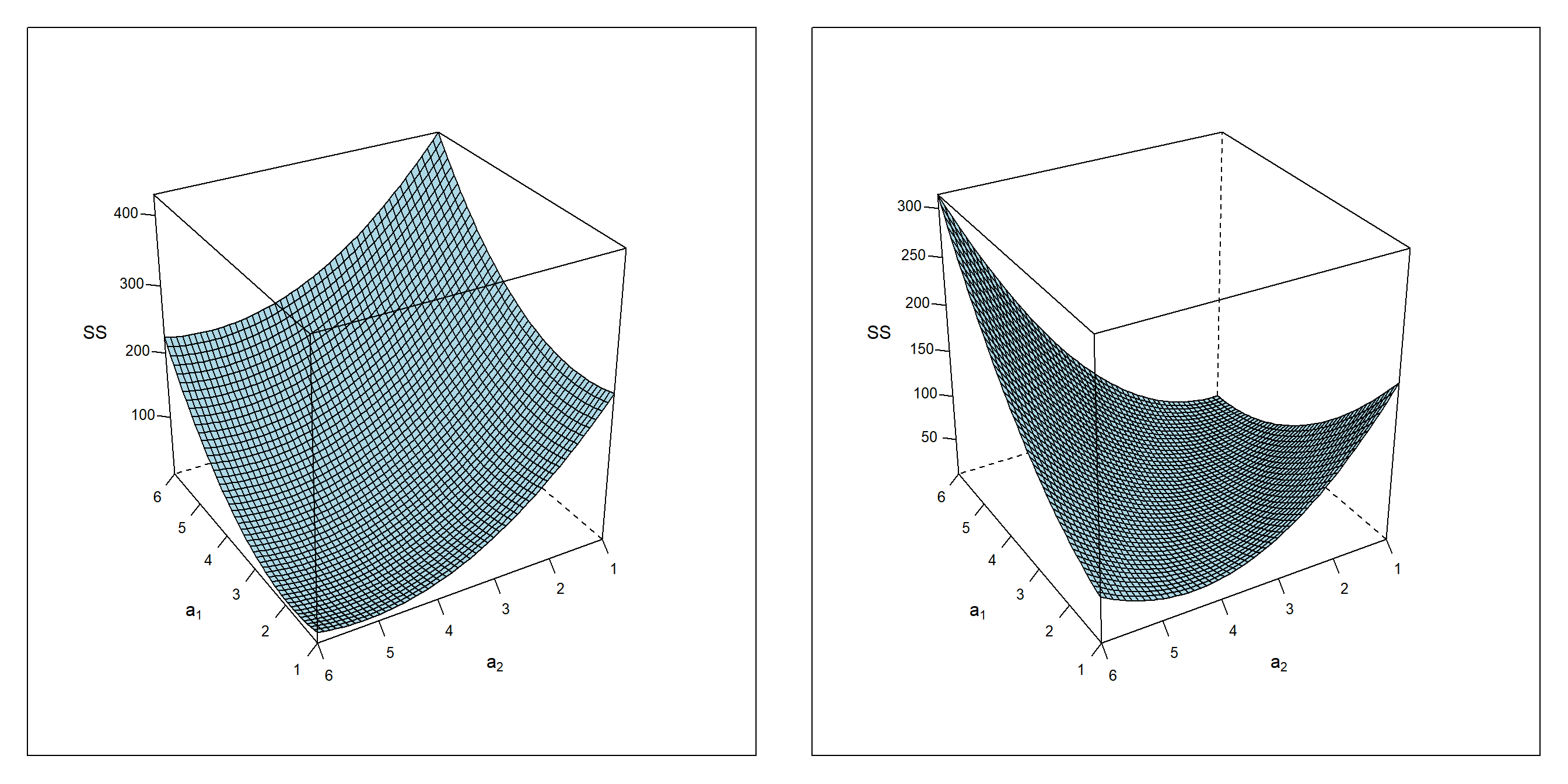
Figure 4.2: \(SS = f(a_{1},a_{2}|a_{0})\) given \(a_{0,design1}=3.194\) (left panel) and \(a_{0,design2}=3.154\) (right panel)
While SS(a1,a2) of design1 reveals a distinct minimum close to the true values at a1=2 and a2=5, the SS(a1,a2) topology of design2 turns out degenerated in one direction but convex and non-degenerated perpendicular to that direction. The degenerated direction in parameter space, figure 4.2, corresponds to directions unpopulated by data in figure 4.1 with the consequence of making the location of the OLS minimum uncertain. More generally, a flat topology in SS(a1,a2) always indicates areas of uncertainty with large standard error, while sharp and convex minima in SS give rise to higher certainty about the location of the minimum thus shrinking the standard error.
While design2 is ill-conditioned but still estimable, the limiting case shown in figure 4.3 is singular and non-estimable. Here, x1 is an exactly linear function of x2, formally x1=b0 + b1x2 with the consequence of rendering the regression equation y=a0 + a1x1 + a2x2 non-estimable. Parameter estimation with a singular design shown in figure 4.3 amounts to the attempt of placing a regression plane onto a one-dimensional data edge which is clearly impossible. Formally, the regression equation y=a0 + a1x1 + a2x2 collapses with the contraint x1=b0 + b1x2 into y=a0 + a1(b0 + b1x2) + a2x2, and the two-dimensional problem degenerates into a one-dimensional regression problem y=c0 + c1x2 with c0=a0+a1b0 and c1=a2+a1b1.

Figure 4.3: Degenerated design for estimating the OLS model \(\hat y=a_{0} + a_{1} \cdot x_{1} + a_{2} \cdot x_{2}\).
Trying to estimate a linear OLS problem y=a0 + a1x1 + a2x2 is equivalent to asking for the independent effects of x1 and x2. When, due to collinearity, no information about the independent effects is available these attempts must fail. Confounding of process factors xi with xk is afflicted with the fundamental problem that in the singular limiting case any linear combination \(a_{1} \cdot x_{1} + a_{2} \cdot x_{2}; \ a_{1},a_{2} \in \mathbb{R}\) is a valid solution of the OLS problem. There are, in other words, an infinite number of solutions for the OLS problem and the collinear data cannot tell one solution from the other. The problem of collinearity becomes worse with increasing number of dimensions and when higher order model terms, such as interactions xixj or square terms xi2, are involved. For instance, it is easy to see that an interaction term xixj will be obscured by collinearity and show up as a quadratic term xi2 due to the confounding constraint \(x_{j} \approx a_{i} \cdot x_{i}\). For these reasons it is virtually impossible to estimate interactions from historical data as there will always be linear dependencies in the data invalidating such attemps.
Confounding can also be the source of paradoxes leading to contradictions between t- and F-test. Consider therefore the following ill-conditioned case with the factors x1,x2 being highly counfounded (rx1,x2 = +0.987).
rm(list=ls())
set.seed(12556)
x <- data.frame(x1=seq(-1,1,length=4))
x$x2 <- x$x1 + rnorm(nrow(x),0,0.1)
x <- rbind(x,x,x)
x$y <- 3 + 2*x$x1 + 5*x$x2 + rnorm(nrow(x),0,1)
summary(lm(y~x1+x2,data=x))
##
## Call:
## lm(formula = y ~ x1 + x2, data = x)
##
## Residuals:
## Min 1Q Median 3Q Max
## -1.2375 -0.6452 0.2270 0.6547 1.1735
##
## Coefficients:
## Estimate Std. Error t value Pr(>|t|)
## (Intercept) 3.0239 0.3479 8.691 1.14e-05 ***
## x1 0.7088 2.2483 0.315 0.7598
## x2 6.2079 2.4621 2.521 0.0327 *
## ---
## Signif. codes: 0 '***' 0.001 '**' 0.01 '*' 0.05 '.' 0.1 ' ' 1
##
## Residual standard error: 0.9281 on 9 degrees of freedom
## Multiple R-squared: 0.9721, Adjusted R-squared: 0.9659
## F-statistic: 157 on 2 and 9 DF, p-value: 1.006e-07In this pathological example the F-test is found highly significant with an F-value of F=157 and DF1=2, DF2=9, however hardly any parameter a1, a2 can be judged significant based on the t-test. On the F-level the model is significant, however on the parameter level it is not significant. This ostensible contradiction can be resolved by remembering that OLS aims at estimating independent effects. However, when there is no information about the independent effects, then the estimates become arbitrary and there are arbitrarily many parameter combinations explaining the response with small error (note R2=0.97).
The problems just discussed are solid reasons motivating DoE, as DoE will avoid confounding in the design phase and thereby render the parameter estimates \(\hat {\beta}\) maximal informative24. Confounding problems can be identified by analysing the correlation structure of the design matrix X. For instance, if two or more columns in X are highly correlated, then OLS estimates will likely be unstable, and the standard error of the collinear parameters will become inflated.
Analysing the confounding structure of large design matrices X with bivariate correlation analyses can be difficult and tedious, especially when there are multicollinear dependencies25 in the design. The condition number \(\kappa\) is a quality score of the design based on the eigenvalue decomposition of the covariance matrix \(\boldsymbol {X^T \cdot X}\) and works even in the presence of multicollinearities. The condition number \(\kappa\) is defined as the ratio of the largest divided by the smallest eigenvalues of \(\boldsymbol {X^T \cdot X}\), \(\kappa = \frac {\lambda_{max} } {\lambda_{min} }; \lambda_{min}>0\), i.e. the ratio of the largest divided by the smallest spread of data in k-dimensional space. Informally, it is a measure of the hyperellipticity or conversely the design’s deviation from hypersphericity (see figure 4.4 for a two-dimensional example). By requiring \(\lambda_{min}>0\), \(\kappa\) measures closeness to singularity and not singularity, and that property can make \(\kappa\) misleading when applied to model matrices with n.col>n.row (see the section on screening designs below for an example). \(\kappa\) is a positive number in the range \(\{ 1, \infty \}\). \(\kappa=1\) indicates a perfectly orthogonal, hypersherical design, while \(\kappa=\infty\) signals a degenerated and almost singular design.
The following R-code shows some examples of how \(\kappa\) can be used for checking design and model quality. Note that \(\kappa\) should always be calculated based on scaled data, and the R-function model.matrix(…,data=data.frame(scale(…))) is the preferred method for doing so (see the R-code below). Figure 4.4 illustrates \(\kappa\) in two dimensions.
set.seed(123)
x <- expand.grid(x1=seq(-1,1,length=5),
    x2=seq(-1,1,length=5)) # orthogonal 5x5 full-factorial
kappa(model.matrix(~x1 + x2 ,
    data=data.frame(scale(x)))) # perfect kappa=1
## [1] 1.01384x$x3 <- x$x1 + x$x2 + rnorm(nrow(x), 0,0.1)
kappa(model.matrix(~x1 + x2 + x3,
data=data.frame(scale(x)))) # collinear kappa=38## [1] 37.7213x$y = 5 + 3*x$x1 + 5*x$x2 - 10*x$x3 +
rnorm(nrow(x), 0,1) # make response
summary(res <- lm(y~x1+x2+x3, data=x) )##
## Call:
## lm(formula = y ~ x1 + x2 + x3, data = x)
##
## Residuals:
## Min 1Q Median 3Q Max
## -1.6026 -0.6389 -0.1808 0.6001 1.4534
##
## Coefficients:
## Estimate Std. Error t value Pr(>|t|)
## (Intercept) 5.11465 0.16693 30.640 < 2e-16 ***
## x1 -0.08703 1.92135 -0.045 0.96430
## x2 1.25674 1.94548 0.646 0.52529
## x3 -6.24715 1.99908 -3.125 0.00512 **
## ---
## Signif. codes: 0 '***' 0.001 '**' 0.01 '*' 0.05 '.' 0.1 ' ' 1
##
## Residual standard error: 0.834 on 21 degrees of freedom
## Multiple R-squared: 0.9809, Adjusted R-squared: 0.9781
## F-statistic: 359 on 3 and 21 DF, p-value: < 2.2e-16kappa(res) # kappa = 46## [1] 45.80286kappa(model.matrix(~x1 + x2 + x3,
data=data.frame(scale(x))) ) # kappa = 38; ## [1] 37.7213round(cor(x),2)## x1 x2 x3 y
## x1 1.00 0.00 0.70 -0.77
## x2 0.00 1.00 0.71 -0.61
## x3 0.70 0.71 1.00 -0.98
## y -0.77 -0.61 -0.98 1.00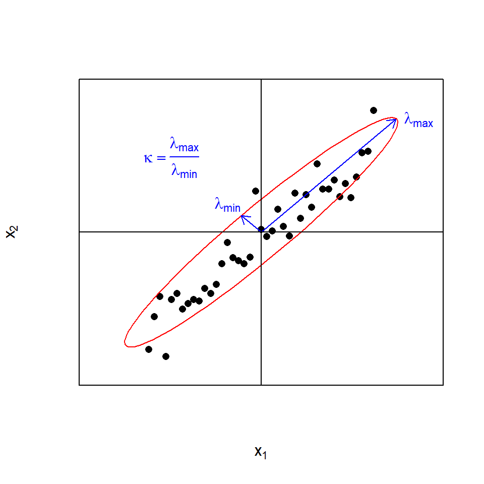
Figure 4.4: The condition number \(\kappa\) as a measure of the (hyper)ellipticity of the data illustrated in two dimensions \(x_{1}\) and \(x_{2}\)
4.2 Mixed level full factorial designs
Mixed level full factorial designs are not an overwhelmingly important design class in chemistry, but they are nevertheless of value as the basis of other important design classes such as the 22-full factorial designs or as candidate designs for optimal designs, an important design class discussed later.
In the following examples mixed-level factorial designs will be used to introduce the ANOVA26 and ANCOVA27 model class, models with either all X-variables entirely categorial or of mixed categorial-numerical data type.
Then, what is a mixed-level full factorial design?
Given factor x1, x2… xI on l1, l2 …lI factor levels, a mixed factorial design is created by combining all factor levels with \(N=l_{1} \cdot l_{2} \cdot ... l_{I} = \prod_{i=1}^{^I} l_{i}\) combinations in total. This defines a grid in I-dimensional space \(\mathbb{R^I}\), hence these designs are alternatively called grid designs. In R such designs can be easily created with base function expand.grid().
As a first example of a mixed-level factorial design consider the following ANOVA problem: A researcher wants to study the performance (here labelled activity) of three different catalysts, cat={A,B,C} and two co-catalyst, co.cat={co1,co2}. The corresponding 3x2 grid is replicated three times making a total of 18 runs. With the indicator function I(TRUE)=1, I(FALSE)=0, the activity is assumed to relate to cat and co.cat by the assumed example model \[activity=1 \cdot I(cat=A) + 2 \cdot I(cat=B) + 3 \cdot I(cat=C) - 1 \cdot I(co.cat=co1) \] \[ +1 \cdot I(co.cat=co2) + 5 \cdot I(cat=A \ \& \ co.cat=co1) + \epsilon ; \epsilon \sim N(0,\sigma=1)\] The R-code creating design, model, and model diagnostics is as follows
rm(list=ls())
set.seed(1234)
x <- expand.grid(cat=c("A","B","C"),
                 co.cat=c("co1","co2")) # factorial 3x2 design
x <- rbind(x,x,x) # make a triple replicate
x <- x[order(runif(nrow(x))),]  # randomize
x$activity <- round( 1*(x$cat=="A") + 2*(x$cat=="B") +
3*(x$cat=="C") - # marginal cat effects
1*(x$co.cat=="co1") +1*(x$co.cat=="co2")   +
# marginal co.cat effects
5*( (x$cat=="A")&(x$co.cat=="co1")) + # interaction
rnorm(nrow(x),0,1) ,4 ) # error term; sigma=1
sapply(x,class)
## cat co.cat activity
## "factor" "factor" "numeric"# check x
rownames(x) <- NULL
knitr::kable(
x, booktabs = TRUE,row.names=T,align="c",
caption = 'A 3x2 mixed level factorial design as basis of
a two-way ANOVA model with interaction'
)| cat | co.cat | activity | |
|---|---|---|---|
| 1 | A | co1 | 4.1100 |
| 2 | A | co1 | 4.5228 |
| 3 | B | co1 | 0.0016 |
| 4 | C | co2 | 3.2237 |
| 5 | A | co1 | 5.0645 |
| 6 | B | co2 | 3.9595 |
| 7 | C | co1 | 1.8897 |
| 8 | A | co2 | 1.4890 |
| 9 | C | co2 | 3.0888 |
| 10 | C | co1 | 1.1628 |
| 11 | B | co1 | 3.4158 |
| 12 | A | co2 | 2.1341 |
| 13 | C | co2 | 3.5093 |
| 14 | C | co1 | 1.5595 |
| 15 | B | co2 | 3.4596 |
| 16 | A | co2 | 1.3063 |
| 17 | B | co2 | 1.5518 |
| 18 | B | co1 | 1.5748 |
summary(res <- lm(activity~(cat+co.cat)^2 , data=x)) # lm model##
## Call:
## lm(formula = activity ~ (cat + co.cat)^2, data = x)
##
## Residuals:
## Min 1Q Median 3Q Max
## -1.6625 -0.2989 -0.0466 0.4401 1.7517
##
## Coefficients:
## Estimate Std. Error t value Pr(>|t|)
## (Intercept) 4.5658 0.5339 8.551 1.89e-06 ***
## catB -2.9017 0.7551 -3.843 0.002340 **
## catC -3.0284 0.7551 -4.011 0.001728 **
## co.catco2 -2.9226 0.7551 -3.871 0.002226 **
## catB:co.catco2 4.2489 1.0679 3.979 0.001830 **
## catC:co.catco2 4.6592 1.0679 4.363 0.000923 ***
## ---
## Signif. codes: 0 '***' 0.001 '**' 0.01 '*' 0.05 '.' 0.1 ' ' 1
##
## Residual standard error: 0.9248 on 12 degrees of freedom
## Multiple R-squared: 0.6836, Adjusted R-squared: 0.5517
## F-statistic: 5.185 on 5 and 12 DF, p-value: 0.009165anova(res) # ANOVA analysis of the model terms## Analysis of Variance Table
##
## Response: activity
## Df Sum Sq Mean Sq F value Pr(>F)
## cat 2 2.1973 1.0986 1.2846 0.312229
## co.cat 1 0.0098 0.0098 0.0115 0.916403
## cat:co.cat 2 19.9649 9.9824 11.6721 0.001532 **
## Residuals 12 10.2629 0.8552
## ---
## Signif. codes: 0 '***' 0.001 '**' 0.01 '*' 0.05 '.' 0.1 ' ' 1# interpretation of OLS
ols.est <- c(
intercept = round(mean(x$activity[x$cat=="A" & x$co.cat=="co1"] ), 4),
catB = round(mean(x$activity[x$cat=="B" & x$co.cat=="co1"] )-
mean(x$activity[x$cat=="A" & x$co.cat=="co1"] ), 4),
catC = round(mean(x$activity[x$cat=="C" & x$co.cat=="co1"] )-
mean(x$activity[x$cat=="A" & x$co.cat=="co1"] ),4),
co.catco2= round(mean(x$activity[x$cat=="A" & x$co.cat=="co2"] ) -
mean(x$activity[x$cat=="A" & x$co.cat=="co1"] ), 4),
catB_co.catco2= round((mean(x$activity[x$cat=="B" & x$co.cat=="co2"])-
mean(x$activity[x$cat=="A" & x$co.cat=="co2"] ))-
(mean(x$activity[x$cat=="B" & x$co.cat=="co1"] )-
mean(x$activity[x$cat=="A" & x$co.cat=="co1"] ) ),4),
catC_co.catco2= round((mean(x$activity[x$cat=="C" & x$co.cat=="co2"] )-
mean(x$activity[x$cat=="A" & x$co.cat=="co2"] )) -
(mean(x$activity[x$cat=="C" & x$co.cat=="co1"] ) -
mean(x$activity[x$cat=="A" & x$co.cat=="co1"] ) ),4)
)
data.frame(ols.est) # print## ols.est
## intercept 4.5658
## catB -2.9017
## catC -3.0284
## co.catco2 -2.9226
## catB_co.catco2 4.2489
## catC_co.catco2 4.6592par(mfrow=c(1,2))
plot(predict(res),rstudent(res),type="n",
ylab="studentized residuals", xlab="predicted response")
text(predict(res),rstudent(res),label=1:nrow(x))
abline(h=0)
grid()
plot(1:nrow(x),rstudent(res),type="n",
ylab="studentized residuals", xlab="run order")
text(1:nrow(x),rstudent(res),label=1:nrow(x))
abline(h=0)
grid() 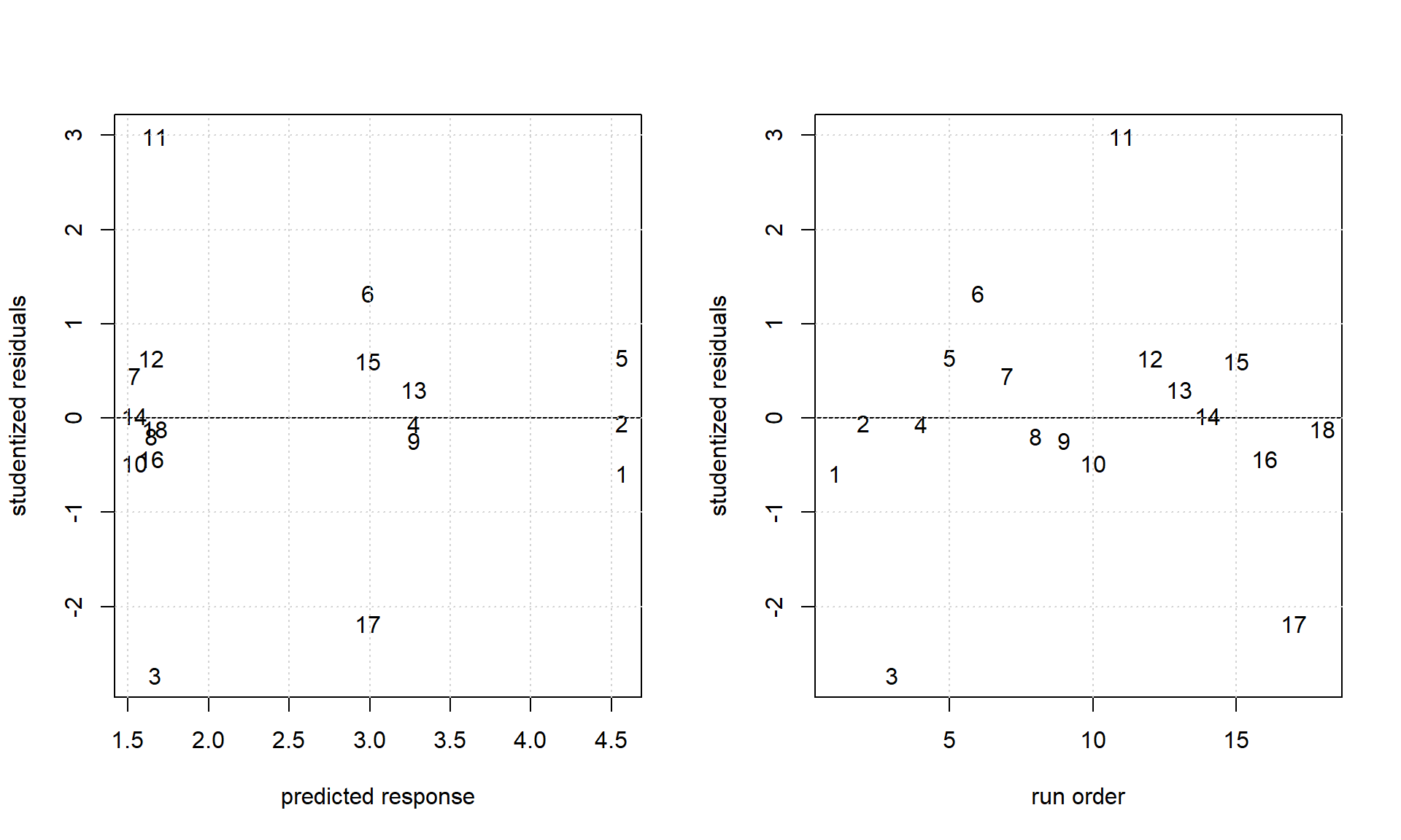
Figure 4.5: Some model diagnostics of the ANOVA model written in R-formula notation as activity ~ (cat + co.cat)^2.
The six OLS parameters from the two-way ANOVA can be interpreted as follows
- Intercept: It is the mean average of the reference group, mean(activity|cat=“A” & co.cat=“co1”)=4.5658.
- catB: It is the mean contrast B-A with co.cat at level “co1”, i.e. mean(activity|cat=“B”&co.cat=“co1”)- mean(activity|cat=“A”&co.cat=“co1”)=-2.9017.
- catC: Likewise follows mean(activity|cat=“C”&co.cat=“co1”) - mean(activity|cat=“A”&co.cat=“co1”)=-3.0284.
- co.catco2: It is the mean constrast co2-co1 given cat at reference A, namely mean(activity|cat=“A”&co.cat=“co2”) - mean(activity|cat=“A”&co.cat=“co1”)= -2.9226.
- catB:co.catco2: The interaction term can be interpreted as the contrast (B-A|co2) - (B-A|co1)= 4.2489 and so quantifies the heterogeneity of the first order contrast B-A over co.cat.
- catC:co.catco2: Analog to #5 follows the interaction contrast (C-A|co2) - (C-A|co1)= 4.6592.
Model interpretation here is already quite complex with the OLS estimators expressed as conditional contrasts of the response activity. However, these conditional contrasts do not nescessarily agree with the contrasts of scientific interest, and it is therefore recommended to refrain from parameter interpretation of ANOVA models and to specify the contrasts of interest directly with some auxiliary functions in R.
For instance, the expected value of the six treatment cells cat*co.cat can be estimated together with test statistics, and from these so called Least-Squares-Means (LSM) all \(\frac {6 \cdot 5} {2} = 15\)28 treatment constrast can be calculated. Least-Squares-Means, contrasts and LSM-plots can be obtained with the following r-code based on the OLS model.
library(plotrix)
x <- data.frame(lsmeans::lsmeans(res,~cat*co.cat)  ) # lsmeans
pairs(emmeans::emmeans(res,~cat*co.cat)) # all contrasts
## contrast estimate SE df t.ratio p.value
## A,co1 - B,co1 2.9017 0.755 12 3.843 0.0221
## A,co1 - C,co1 3.0284 0.755 12 4.011 0.0167
## A,co1 - A,co2 2.9226 0.755 12 3.871 0.0211
## A,co1 - B,co2 1.5755 0.755 12 2.086 0.3544
## A,co1 - C,co2 1.2918 0.755 12 1.711 0.5500
## B,co1 - C,co1 0.1267 0.755 12 0.168 1.0000
## B,co1 - A,co2 0.0209 0.755 12 0.028 1.0000
## B,co1 - B,co2 -1.3262 0.755 12 -1.756 0.5243
## B,co1 - C,co2 -1.6099 0.755 12 -2.132 0.3339
## C,co1 - A,co2 -0.1058 0.755 12 -0.140 1.0000
## C,co1 - B,co2 -1.4530 0.755 12 -1.924 0.4337
## C,co1 - C,co2 -1.7366 0.755 12 -2.300 0.2655
## A,co2 - B,co2 -1.3472 0.755 12 -1.784 0.5089
## A,co2 - C,co2 -1.6308 0.755 12 -2.160 0.3218
## B,co2 - C,co2 -0.2836 0.755 12 -0.376 0.9988
##
## P value adjustment: tukey method for comparing a family of 6 estimatesx <- x[order(x$cat,x$co.cat),]
x## cat co.cat lsmean SE df lower.CL upper.CL
## 1 A co1 4.565767 0.5339293 12 3.4024347 5.729099
## 4 A co2 1.643133 0.5339293 12 0.4798014 2.806465
## 2 B co1 1.664067 0.5339293 12 0.5007347 2.827399
## 5 B co2 2.990300 0.5339293 12 1.8269680 4.153632
## 3 C co1 1.537333 0.5339293 12 0.3740014 2.700665
## 6 C co2 3.273933 0.5339293 12 2.1106014 4.437265p.x <- rep(c(0.9,1.1),3)+ rep(0:2,each=2)
plot(p.x,x$lsmean,type="p",pch=16,col=rep(c("red","blue"),3),axes=F,
xlab="cat",ylab="Least-Square-Means", ylim=c(min(x$lower.CL),max(x$upper.CL) ))
axis(1,at=1:3,labels=LETTERS[1:3])
axis(2)
plotCI(p.x,x$lsmean,ui=x$upper.CL,li=x$lower.CL,
err="y",add=TRUE,pch=" ",col=rep(c("red","blue"),3), gap=0)
grid()
box()
legend("top",c("co.cat","co1","co2"),text.col=c("black","red","blue"))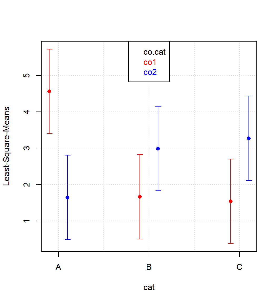
Figure 4.6: Interaction plot cat|co.cat
The combination cat=“A” and co.cat=“co1” sticks out significantly thereby indicating a positive synergism between cat=“A” and co.cat=“co1”.
Historically, problems with all predictors being categorial and responses continuous are called ANalysis Of VAriance (ANOVA) and deal with estimating and comparing many mean values. Multiway-ANOVA (in the example: two-way ANOVA) can be conceived as a multidimensional generalization of the two-sample t-test within the framework of OLS.
Between multiple regression with all X-variables and responses continuous and ANOVA lies the ANalysis of COVAriance (ANCOVA) method with predictors being a mix of continuous and categorial factors. As the following example will show, ANCOVA problems can be treated conveniently within the framework of OLS. In the above example, a strong and significant synergism between cat=“A” and co.cat=“co1” was observed. In the ANOVA set-up the co.cat-concentration was held constant at co.catco1= 1% for all cats. In a follow-up experiment the co.catco1 concentration is varied in the range co1={1,3%} on 5 levels for the three catalysts, cat={A,B,C} and the activity of the 3x5 factorial design was measured. For the purpose of demonstration the “true” model is given by the linear model \[activity = 5 \cdot I(cat=A) - 1 \cdot I(cat=B) - 2 \cdot I(cat=C) \] \[ - 1 \cdot I(cat=A) \cdot co.cat + 2 \cdot I(cat=B) \cdot co.cat + 3 \cdot I(cat=C) \cdot co.cat + \epsilon; \] \[ \epsilon \sim N(0,1)\] The data is depicted in figure 4.7 and listed in table 4.3 along with the outcome of the joint ANCOVA OLS-analysis activity ~ (cat+co.cat)2.29
rm(list=ls())
set.seed(123)
library(ggplot2)

x <- data.frame(cat=rep(LETTERS[1:3],each=5),
            co.cat=rep(seq(1,3,length=5), 3)  )
x  <- x[order(runif(nrow(x))), ]
rownames(x) <- NULL
x$activity <- 5*(x$cat=="A")  -1*(x$cat=="B") +
       -2*(x$cat=="C") - 1*(x$cat=="A")*x$co.cat +
       2*(x$cat=="B")*x$co.cat +  3*(x$cat=="C")*x$co.cat +
  rnorm(nrow(x),0,1)
knitr::kable(
  x, booktabs = TRUE,row.names=T, digits=3,align="c",
  caption = '3x5 cat x co.cat design for estimating the
joint model activity ~ (cat+co.cat)\\^2 with OLS')| cat | co.cat | activity | |
|---|---|---|---|
| 1 | B | 1.0 | 2.281 |
| 2 | C | 3.0 | 5.273 |
| 3 | A | 1.0 | 5.690 |
| 4 | A | 2.0 | 3.504 |
| 5 | C | 1.5 | 5.028 |
| 6 | B | 3.0 | 5.549 |
| 7 | B | 1.5 | 2.238 |
| 8 | B | 2.5 | 2.951 |
| 9 | C | 2.5 | 6.795 |
| 10 | C | 2.0 | 4.826 |
| 11 | A | 1.5 | 3.444 |
| 12 | A | 2.5 | 1.716 |
| 13 | B | 2.0 | 2.266 |
| 14 | A | 3.0 | 1.784 |
| 15 | C | 1.0 | 0.665 |
ggplot(data = x, aes(x = co.cat, y = activity, colour = cat)) +
    geom_smooth(method="lm", se=F) + geom_point() + theme_bw()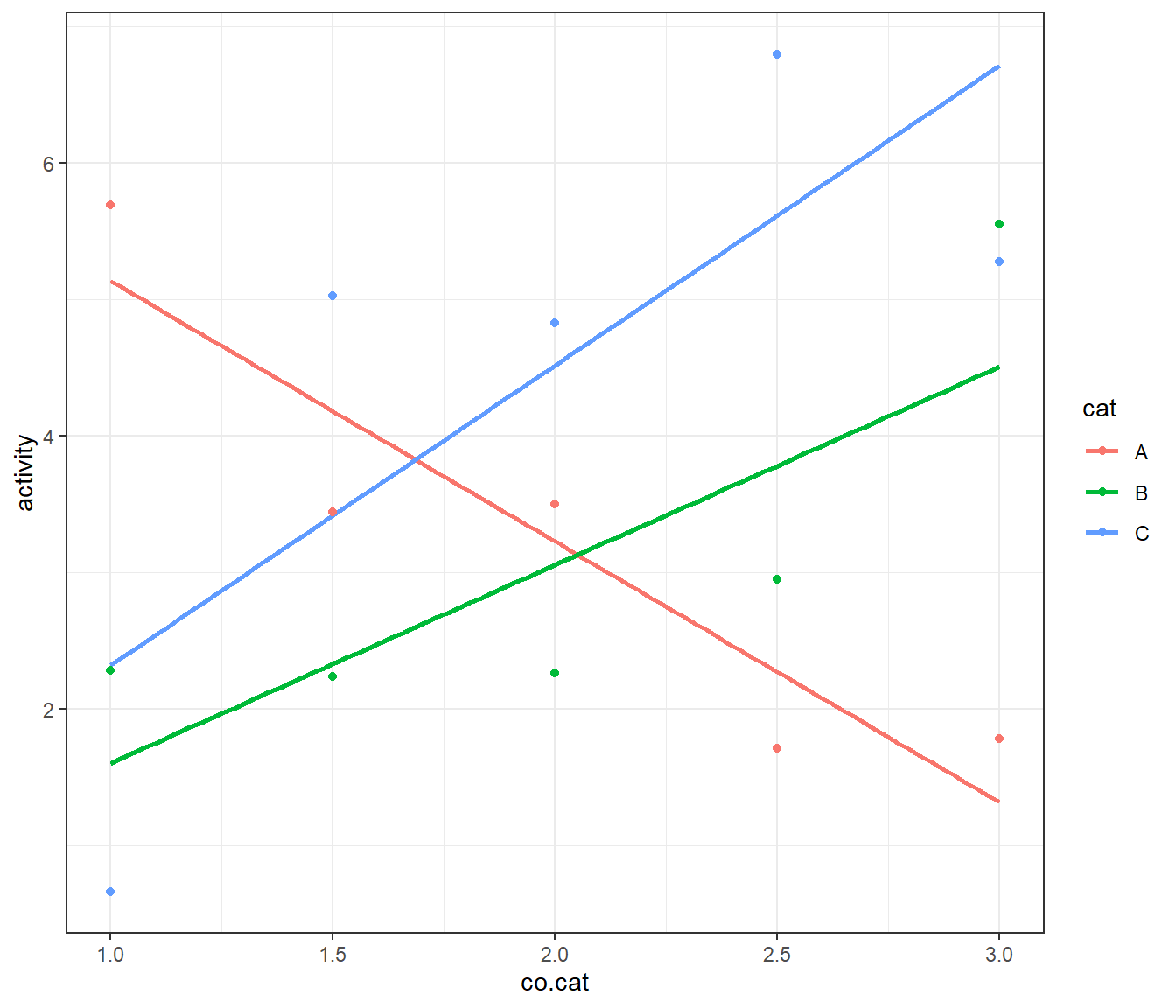
Figure 4.7: Plot of activity ~ co.cat by cat of the ANCOVA example
summary(res <- lm(activity~(cat + co.cat)^2, data=x))##
## Call:
## lm(formula = activity ~ (cat + co.cat)^2, data = x)
##
## Residuals:
## Min 1Q Median 3Q Max
## -1.6559 -0.7640 0.2762 0.6139 1.6092
##
## Coefficients:
## Estimate Std. Error t value Pr(>|t|)
## (Intercept) 7.0439 1.6255 4.333 0.0019 **
## catB -6.8868 2.2988 -2.996 0.0151 *
## catC -6.9193 2.2988 -3.010 0.0147 *
## co.cat -1.9082 0.7663 -2.490 0.0344 *
## catB:co.cat 3.3582 1.0837 3.099 0.0127 *
## catC:co.cat 4.1045 1.0837 3.788 0.0043 **
## ---
## Signif. codes: 0 '***' 0.001 '**' 0.01 '*' 0.05 '.' 0.1 ' ' 1
##
## Residual standard error: 1.212 on 9 degrees of freedom
## Multiple R-squared: 0.7128, Adjusted R-squared: 0.5533
## F-statistic: 4.468 on 5 and 9 DF, p-value: 0.02527With factor level A being the reference, the reported estimates are contrasts against the reference, here \(\Delta a_{i} = a_{i} - a_{A}\). Keeping this in mind, the regression model reads \[activity=a_{0} + \Delta a_{0,B} \cdot I(cat=B) + \Delta a_{0,C} \cdot I(cat=C) + a_{1}\cdot co.cat \] \[ + \ \Delta a_{1,B} \cdot I(cat=B) \cdot co.cat + \Delta a_{1,C} \cdot I(cat=C) \cdot co.cat \] From the above OLS estimates unbiased estimates of, say, B can be obtained with \[activity_{B}(co.cat) = a_{0} + \Delta_{0,B} + (a_{1} + \Delta a_{1,B} ) \cdot co.cat \] \[ = 7.0439-6.8868 + (-1.9082+3.3582) \cdot co.cat \] \[ = 0.1571 + 1.45 \cdot co.cat\] which is within standard error in agreement with the model having generated the data30.
It is worthwhile comparing the joint ANCOVA analysis with the results from OLS analysis stratified by cat31. OLS results of linear regression analysis stratified by cat are summarized in table 4.4. Stratified analysis yields the same location parameter as the joint ANCOVA analysis, however the ANCOVA test statistics is different and more powerful, as there are more degrees of freedom for estimating the error variance (DFANCOVA=9; DFstratified=3). This will render the ANCOVA error variance smaller compared to the stratified results, hence smaller effects can be detected with the joint ANCOVA model. Joint model analysis of data is usually superior to stratified data analysis in terms of power and usually less laborious than stratified analysis. Joint modeling should therefore be the method of first choice when analysing complex designs.
| Parameter | cat | Estimate | Std. Error | t value | Pr(>|t|) |
|---|---|---|---|---|---|
| Intercept | A | 7.0439 | 0.9342 | 7.5400 | 0.0048 |
| co.cat | A | -1.9082 | 0.4404 | -4.3329 | 0.0227 |
| Intercept | B | 0.1571 | 1.3108 | 0.1199 | 0.9122 |
| co.cat | B | 1.4500 | 0.6179 | 2.3466 | 0.1006 |
| Intercept | C | 0.1246 | 2.3100 | 0.0539 | 0.9604 |
| co.cat | C | 2.1963 | 1.0889 | 2.0170 | 0.1371 |
4.3 Full factorial 2K designs
Full factorial 2K designs are a subclass of the above grid designs with all K-factors on two levels only. 2K factorials are an important design class, because from these designs many other designs can be derived such as screening designs, fractional factorial designs, and central composite designs, all to be discussed later in more detail. The levels of the factors x1, x2 …xK are usually given in coded units, {-1,+1} with -1 and +1 denoting the lower and upper bounds of the K-factors. A simple 2^3 full factorial for the factors x1, x2 and x3 is depicted in figure 4.8
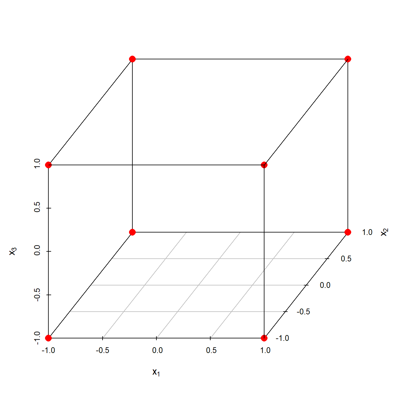
Figure 4.8: \(2^3\) full factorial design with factorial points labelled red
Full factorial 2K designs span a K-dimensional sphere \(\mathbb{R^k}\), these are squares in two, cubes in three and hypercubes in K>3 dimensions, with 2K vertex points of the K-cube.
It can be shown that full factorial designs provide support for estimating all linear effects and all K-way interactions, schematically written \[y=\sum {(\text{1-way}), (\text{2-way}),(\text{3-way}),...(\text{K-way})}\] with 1-way interaction denoting main effects xi, 2-way bilinear terms xixj, 3-way trilinear terms xixjxk etc. up to K-way term x1x2x3…xK. Given K factors the number of k-way interaction terms can be calculated with the well known combinatorial expression (4.1).
Summing up over all interactions is equal to the number of support points of the 2K design and given by equation (4.2)
\[\begin{equation} \sum_{k=1}^K{{K} \choose {k} } = 2^K \tag{4.2} \end{equation}\]The linear model supported by a 24 design can thus be expressed by the lengthy expression \[y=a_{0}+a_{1}\cdot x_{1} +a_{2}\cdot x_{2}+a_{3}\cdot x_{3}+a_{4}\cdot x_{4} + \] \[ a_{12}\cdot x_{1}\cdot x_{2} + a_{13}\cdot x_{1}\cdot x_{3}+ a_{14}\cdot x_{1}\cdot x_{4}+ a_{23}\cdot x_{2}\cdot x_{3}+ a_{24}\cdot x_{2}\cdot x_{4}+ a_{34}\cdot x_{3}\cdot x_{4} + \] \[ a_{123} \cdot x_{1}\cdot x_{2} \cdot x_{3} + a_{124} \cdot x_{1}\cdot x_{2} \cdot x_{4} + a_{234} \cdot x_{2}\cdot x_{3} \cdot x_{4} + a_{134} \cdot x_{1}\cdot x_{3} \cdot x_{4} + \] \[ a_{1234} \cdot x_{1} \cdot x_{2} \cdot x_{3} \cdot x_{4} + \epsilon\]
There are four main effects, ten 2-way interactions, four 3-way interactions and one 4-way interaction being supported by 16 ( 24) design points, so there are 16 model parameters to be estimated from 16 runs. When the number of runs N equals the number of regression parameters p, the design is called saturated. Such designs are estimable, however they have no degrees of freedom for estimating the error variance, hence OLS will always fit the data with R2=1 similar to fitting a line with two support points only.
Based on the Taylor series expansion, these complex expressions can be simplified. Given any smooth and continuous function f(), the higher order terms of the Taylor series expansion will vanish, and this fundamental property is being exploited by assuming the higher order terms >2-way to be zero or close to zero. With this assumption, all interaction terms>2 \(\approx 0\), the model equation from above becomes \[y=a_{0}+a_{1}\cdot x_{1} +a_{2}\cdot x_{2}+a_{3}\cdot x_{3}+a_{4}\cdot x_{4} + \] \[ a_{12}\cdot x_{1}\cdot x_{2} + a_{13}\cdot x_{1}\cdot x_{3}+ a_{14}\cdot x_{1}\cdot x_{4}+ a_{23}\cdot x_{2}\cdot x_{3}+ a_{24}\cdot x_{2}\cdot x_{4}+ a_{34}\cdot x_{3}\cdot x_{4} + \epsilon ; \] \[ \epsilon \sim N(0,\sigma^2) \] usually written in short notation \[y=a_{0}+\sum_{i=1}^4a_{i}\cdot x_{i} + \sum_{j>i}^4a_{ij}\cdot x_{i}\cdot x_{j} + \epsilon\]
In this formula \(\epsilon\) stands either for the effects of the hidden confounders \(\Delta z_K\) and/or the sum of the neglected higher order terms. At any rate, the Central Limit Theorem will “work” towards normalizing these terms into something close to \(\epsilon \sim N(0,\sigma^2)\). Now, the above model, after omitting higher order interactions, becomes a bilinear surrogate model of the true, however unknown function f(), that is \[ f(\Delta x_{1}, \Delta x_{2}... \Delta x_{I}) \approx a_{0} + \sum_{i}a_{i}\cdot x_{i} + \sum_{j>i}a_{ij}\cdot x_{i}\cdot x_{j}\] with p=11 regression parameters, hence there are N-p=5 degrees of freedom for estimating \(\sigma^2\).
The redundancy factor R can be defined as the number of trials N divided by the number of model parameters p, \(R=\frac {N} {p}\). Assuming a bilinear model structure, redundancies R(K) can be calculated for the full factorial designs as a function of the dimension K according to \[R(K)=\frac {2^K} {1+K+ \frac {K\cdot(K-1)} {2} }\] some of which are listed in table 4.5.
| K | Redundancy |
|---|---|
| 2 | 1.00 |
| 3 | 1.14 |
| 4 | 1.45 |
| 5 | 2.00 |
| 6 | 2.91 |
| 7 | 4.41 |
| 8 | 6.92 |
| 9 | 11.13 |
| 10 | 18.29 |
According to table 4.5, a five factor design, 25, has already a redundancy of 2, meaning, that one half of the experimental effort (16 trials) is spend on estimating the error variance. A redundancy of two is probably a number too large for making a 25 design an economical choice under bilinear model assumption.
As a rule of thumb, RK should be in the range \(1 \leq R_{K} \leq 1.5\) with the lower bound indicating a saturated design and the upper value admitting one third of the experimental effort for estimating the error variance. Given this rule, the number of factors suitable for full factorial analysis are restricted to K=2,3,4 with K=4 being the ideal number. The two factor design K=2 is a saturated design requiring additional trials for estimating the error variance. For this and other reasons explained below, full factorial or fractional factorial designs should always be augmented by replicates, usually triple replicates, located at the center of the design because
- Placing replicates in the center will not disturb the balance (orthogonality) of the design while providing an unbiased estimate of the pure replication error of the experimental setup.
- Replicates at the center serve as a check for the presence of convex effects (minima, maxima) and are a base for estimating the sum of the quadratic model terms \(\sum_{i} a_{ii}\), the “global convexity”.
Figure 4.9 shows a 23 design augmented by triple replicates at the center, (0,0,0).
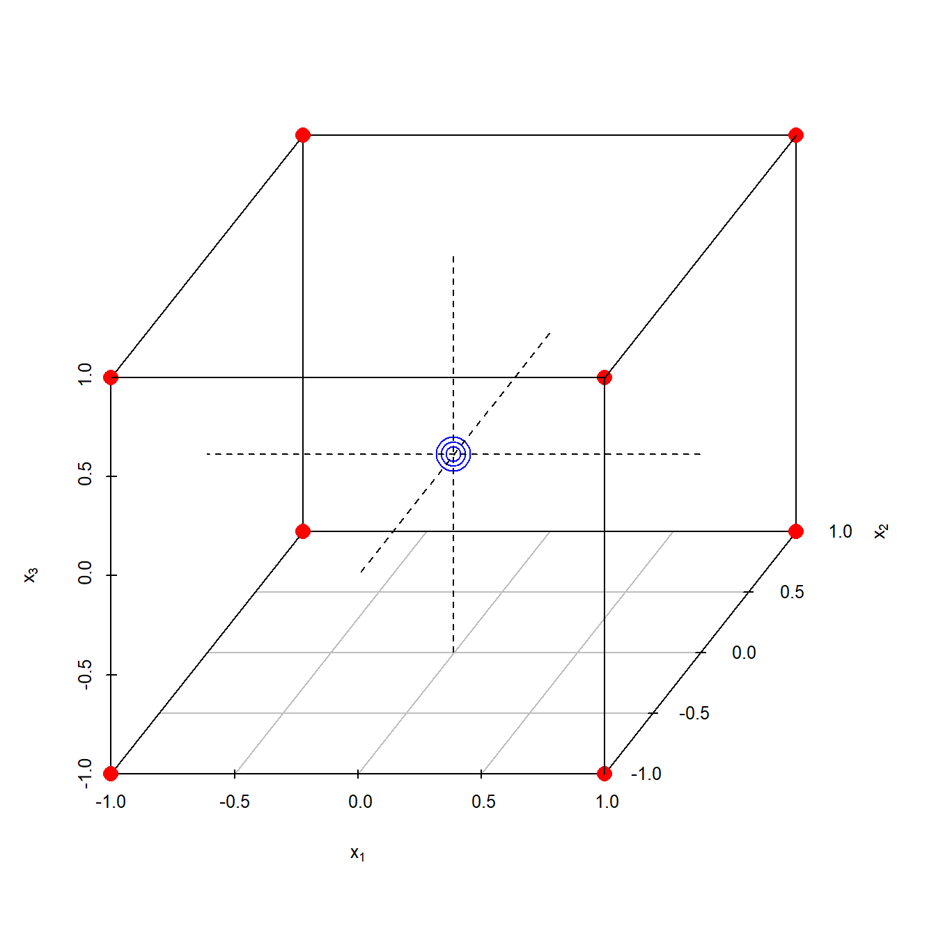
Figure 4.9: \(2^3\) full factorial design with triple replicates marked blue in the center
The discussed concepts become transparent with the following simulation example involving six steps, namely
- A full factorial coded design + three center point is created using the FrF2 function of the library “FrF2”. Note that FrF2 excludes the center points from randomization by placing them at the beginning, middle and end of the design. This optimally supports estimation of serial effects.
- The design is uncoded with a function from the DoE library “rsm” with the linear transformation \(x_{uncoded} = halfway \cdot x_{coded} + center\)
- \(\kappa\) is being calulated for the coded, uncoded and standardized uncoded design showing \(\kappa\) to be highly scale sensitive. Hence, unit variance scaling (“standardization”) is mandatory when using kappa on uncoded data.
- Response y is realized from the assumed true model \(y = 10 + 2 \cdot x_{1} + 3 \cdot x_{2} + 5 \cdot x_{1} \cdot x_{2} + 2 \cdot x_{3}^2 + N(0,1)\)
- The following three OLS models are given in R notation32 and estimated from the data:
- M1: y~(x1+x2+x3+x4)^2;
- M2: y~(x1+x2+x3+x4)^2 + I(x1^2);
- M3: y~(x1+x2+x3+x4)^2 + I(x4^2);
- Residuals for M1 and M2 are depicted in figure 4.10
rm(list=ls())
set.seed(12556)
x <- FrF2::FrF2(nruns=16,nfactors=4,
     factor.names=paste("x",1:4,sep=""), ncenter=3, randomize=F)
## creating full factorial with 16 runs ...x <- as.data.frame(x)
x <- x[order(runif(nrow(x))),]
x.uncoded <- data.frame(rsm::coded.data(x,temp~ 50*x1+100,
cat~4*x2+4, stirrer~100*x3+100, conc~10*x4+10) )# uncode
cbind(x,x.uncoded) # plot coded + uncoded design## x1 x2 x3 x4 temp cat stirrer conc
## 10 1 -1 -1 1 150 0 0 20
## 2 1 -1 -1 -1 150 0 0 0
## 12 1 1 -1 1 150 8 0 20
## 15 -1 1 1 1 50 8 200 20
## 19 0 0 0 0 100 4 100 10
## 5 -1 -1 1 -1 50 0 200 0
## 4 1 1 -1 -1 150 8 0 0
## 18 0 0 0 0 100 4 100 10
## 3 -1 1 -1 -1 50 8 0 0
## 6 1 -1 1 -1 150 0 200 0
## 14 1 -1 1 1 150 0 200 20
## 13 -1 -1 1 1 50 0 200 20
## 8 1 1 1 -1 150 8 200 0
## 7 -1 1 1 -1 50 8 200 0
## 9 -1 -1 -1 1 50 0 0 20
## 11 -1 1 -1 1 50 8 0 20
## 17 0 0 0 0 100 4 100 10
## 16 1 1 1 1 150 8 200 20
## 1 -1 -1 -1 -1 50 0 0 0kappa(model.matrix(~(x1+x2+x3+x4)^2, data=x)) # kappa coded## [1] 1.082183kappa(model.matrix(~(temp +cat +stirrer+ conc)^2,
data=x.uncoded)) # kappa uncoded## [1] 53062.32kappa(model.matrix(~(temp +cat +stirrer+ conc)^2,
data=data.frame(scale(x.uncoded)))) ## [1] 1.02579 # kappa on standardized uncoded data
set.seed(1234)
x$y <- 10 + 2*x$x1 + 3*x$x2 + 5*x$x1*x$x2 +
5*x$x3^2 + rnorm(nrow(x),0,1)
round(cor(model.matrix(~x1+x2+x3+x4+I(x1^2)+I(x2^2)
+I(x3^2)+I(x4^2),data=x)[,-1]),2) # note confounding X^2## x1 x2 x3 x4 I(x1^2) I(x2^2) I(x3^2) I(x4^2)
## x1 1 0 0 0 0 0 0 0
## x2 0 1 0 0 0 0 0 0
## x3 0 0 1 0 0 0 0 0
## x4 0 0 0 1 0 0 0 0
## I(x1^2) 0 0 0 0 1 1 1 1
## I(x2^2) 0 0 0 0 1 1 1 1
## I(x3^2) 0 0 0 0 1 1 1 1
## I(x4^2) 0 0 0 0 1 1 1 1summary(res1 <- lm(y~(x1+x2+x3+x4)^2, data=x))##
## Call:
## lm(formula = y ~ (x1 + x2 + x3 + x4)^2, data = x)
##
## Residuals:
## Min 1Q Median 3Q Max
## -4.3662 0.1089 0.5638 1.0582 1.8634
##
## Coefficients:
## Estimate Std. Error t value Pr(>|t|)
## (Intercept) 13.81952 0.64954 21.276 2.50e-08 ***
## x1 1.99071 0.70782 2.812 0.0228 *
## x2 2.90832 0.70782 4.109 0.0034 **
## x3 -0.30349 0.70782 -0.429 0.6794
## x4 -0.07570 0.70782 -0.107 0.9175
## x1:x2 5.23157 0.70782 7.391 7.68e-05 ***
## x1:x3 -0.02585 0.70782 -0.037 0.9718
## x1:x4 0.13227 0.70782 0.187 0.8564
## x2:x3 -0.17196 0.70782 -0.243 0.8142
## x2:x4 0.02173 0.70782 0.031 0.9763
## x3:x4 -0.37889 0.70782 -0.535 0.6070
## ---
## Signif. codes: 0 '***' 0.001 '**' 0.01 '*' 0.05 '.' 0.1 ' ' 1
##
## Residual standard error: 2.831 on 8 degrees of freedom
## Multiple R-squared: 0.9091, Adjusted R-squared: 0.7955
## F-statistic: 8 on 10 and 8 DF, p-value: 0.00354summary(res2 <- lm(y~(x1+x2+x3+x4)^2 + I(x1^2), data=x))##
## Call:
## lm(formula = y ~ (x1 + x2 + x3 + x4)^2 + I(x1^2), data = x)
##
## Residuals:
## Min 1Q Median 3Q Max
## -1.20396 -0.33077 -0.08242 0.50941 1.10800
##
## Coefficients:
## Estimate Std. Error t value Pr(>|t|)
## (Intercept) 9.79049 0.54768 17.876 4.23e-07 ***
## x1 1.99071 0.23715 8.394 6.70e-05 ***
## x2 2.90832 0.23715 12.264 5.50e-06 ***
## x3 -0.30349 0.23715 -1.280 0.241
## x4 -0.07570 0.23715 -0.319 0.759
## I(x1^2) 4.78447 0.59682 8.017 9.00e-05 ***
## x1:x2 5.23157 0.23715 22.060 9.94e-08 ***
## x1:x3 -0.02585 0.23715 -0.109 0.916
## x1:x4 0.13227 0.23715 0.558 0.594
## x2:x3 -0.17196 0.23715 -0.725 0.492
## x2:x4 0.02173 0.23715 0.092 0.930
## x3:x4 -0.37889 0.23715 -1.598 0.154
## ---
## Signif. codes: 0 '***' 0.001 '**' 0.01 '*' 0.05 '.' 0.1 ' ' 1
##
## Residual standard error: 0.9486 on 7 degrees of freedom
## Multiple R-squared: 0.9911, Adjusted R-squared: 0.977
## F-statistic: 70.63 on 11 and 7 DF, p-value: 4.318e-06summary(res3 <- lm(y~(x1+x2+x3+x4)^2 + I(x4^2), data=x))##
## Call:
## lm(formula = y ~ (x1 + x2 + x3 + x4)^2 + I(x4^2), data = x)
##
## Residuals:
## Min 1Q Median 3Q Max
## -1.20396 -0.33077 -0.08242 0.50941 1.10800
##
## Coefficients:
## Estimate Std. Error t value Pr(>|t|)
## (Intercept) 9.79049 0.54768 17.876 4.23e-07 ***
## x1 1.99071 0.23715 8.394 6.70e-05 ***
## x2 2.90832 0.23715 12.264 5.50e-06 ***
## x3 -0.30349 0.23715 -1.280 0.241
## x4 -0.07570 0.23715 -0.319 0.759
## I(x4^2) 4.78447 0.59682 8.017 9.00e-05 ***
## x1:x2 5.23157 0.23715 22.060 9.94e-08 ***
## x1:x3 -0.02585 0.23715 -0.109 0.916
## x1:x4 0.13227 0.23715 0.558 0.594
## x2:x3 -0.17196 0.23715 -0.725 0.492
## x2:x4 0.02173 0.23715 0.092 0.930
## x3:x4 -0.37889 0.23715 -1.598 0.154
## ---
## Signif. codes: 0 '***' 0.001 '**' 0.01 '*' 0.05 '.' 0.1 ' ' 1
##
## Residual standard error: 0.9486 on 7 degrees of freedom
## Multiple R-squared: 0.9911, Adjusted R-squared: 0.977
## F-statistic: 70.63 on 11 and 7 DF, p-value: 4.318e-06colcol <- rep("black",nrow(x))
colcol[apply(abs(x[,1:4]),1,sum)==0] <- "red"
par(mfrow=c(1,2))
plot(predict(res1), rstudent(res1),
xlab=expression( paste("predicted response ", hat(y)) ) ,
ylab="studentized residuals",type="n",
main=expression(paste("(",frac(paste("y - ",
hat(y)),sigma), ") ~ ", hat(y) )) )
text(predict(res1), rstudent(res1),label=1:nrow(x), col=colcol)
abline(h=c(-2,0,2),lty=c(2,1,2))
plot(predict(res2), rstudent(res2),
xlab=expression( paste("predicted response ", hat(y)) ) ,
ylab="studentized residuals",type="n",
main=expression(paste("(",frac(paste("y - ",
hat(y)),sigma), ") ~ ", hat(y) )) )
text(predict(res2), rstudent(res2),
label=1:nrow(x), col=colcol)
abline(h=c(-2,0,2),lty=c(2,1,2))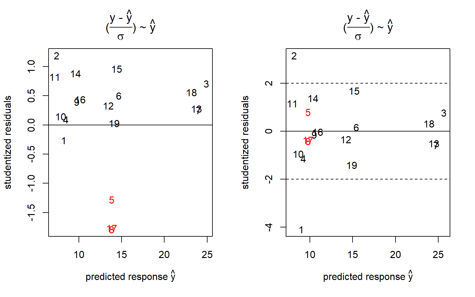
Figure 4.10: Residuals based on the parametric models \(\hat y = (x_{1}+x_{2}+x_{3}+x_{4})^2\) (left panel) and \(\hat y = (x_{1}+x_{2}+x_{3}+x_{4})^2 + x_{1}^2\) (right panel) with center points labelled red
The example is instructive by revealing all four square terms \(x_{i}^2\) confounded with each other (see the correlation analysis of the expanded design matrix). This explains why all models \(y \sim ~(x_{1}+x_{2}+x_{3}+x_{4})^2 + x_{i}^2 ; \ i=1,2,3,4\) will report the same square estimates \(a_{ii}=4.39 \pm 0.37\)33. These modeling results suggest some convexity not being accounted for by the bilinear model M1. The residual plot, figure 4.10, tells a similar story: The residual plot of M1 (left panel) reveals the center points #5,#8,#17 to deviate significantly from the model (the horizontal line) within replication error, thereby indicating the presence of convex effects in the data. On the right panel of figure 4.10 the convex effect is being absorbed (erroneously) by the term \(x_{1}^2\) and #5,#8,#17 are now unbiasedly predicted by M2.
The ambiguities regarding aii2 can be resolved by augmenting the factorial design with star points, a class of trials that will be discussed in more detail in the chapter on RSM designs below.
4.4 Fractional factorial 2K-P designs
Full factorial designs are of limited use for estimating bilinear surrogate models in higher dimension as the design redundany R(K) grows rapidly with dimension K>4. Augmented by center points, full factorial designs can at best be used to economically investigate the effects of two, three or four factors.
High redundancies result from the fact that full factorial designs support higher order effects, here interactions of order >2, which are assumed small and of no scientific interest. Hence, the question arises whether it is possible to omit those points in the design supporting higher order interaction while leaving points supporting 1- and 2-way interactions untouched?
This is in fact possible with a class of designs known as fractional factorial designs, which fill the gap by economically supporting bilinear models of factor dimension K>4.
Fractional factorial designs can be derived analytically from full factorial designs by reassigning higher order interactions to main effects. This will be explained in the following by deriving a five factor resolution 5 design (a 2(5-1) design) from a full factorial 24 design. Table 4.6 lists a 24 design along with its largest possible interaction term the 4-way interaction x1:x2:x3:x434, which is simply the product of the four main effects x1-x4. In total, there are 11 interaction terms in a 24 design which are all orthogonal (i.e. uncorrelated with rPearson=0) to each other. Fractional factorial designs make use of this property by assigning a new factor, here x5, to the highest contrast x1:x2:x3:x4. The confounding properties of this new design can be evaluated easily. From the identity \(x_{5}=x_{1} \cdot x_{2} \cdot x_{3} \cdot x_{4}\) follows by multiplying with \(x_{5}\) the important identity \[ x5 \cdot x5 = I = x1 \cdot x2 \cdot x3 \cdot x4 \cdot x5 \] with I denoting the 1-column. The identity \(\boxed { I = x_{1} \cdot x_{2} \cdot x_{3} \cdot x_{4} \cdot x_{5}}\) is called the defining contrast of the design with the length (or the shortest length when there are several defining contrasts) of the defining contrast(s) being called design resolution (here: resolution=5).
| x1 | x2 | x3 | x4 | x1:x2:x3:x4 |
|---|---|---|---|---|
| -1 | -1 | -1 | -1 | 1 |
| 1 | -1 | -1 | -1 | -1 |
| -1 | 1 | -1 | -1 | -1 |
| 1 | 1 | -1 | -1 | 1 |
| -1 | -1 | 1 | -1 | -1 |
| 1 | -1 | 1 | -1 | 1 |
| -1 | 1 | 1 | -1 | 1 |
| 1 | 1 | 1 | -1 | -1 |
| -1 | -1 | -1 | 1 | -1 |
| 1 | -1 | -1 | 1 | 1 |
| -1 | 1 | -1 | 1 | 1 |
| 1 | 1 | -1 | 1 | -1 |
| -1 | -1 | 1 | 1 | 1 |
| 1 | -1 | 1 | 1 | -1 |
| -1 | 1 | 1 | 1 | -1 |
| 1 | 1 | 1 | 1 | 1 |
With the defining contrast being known, the whole confounding structure of the design can be derived. For instance, in the above 2(5-1) design the main effect of, say, \(x_{1}\) is confounded with the four way term \(\mathbf{x_{1}} = x_{1} \cdot I = x_{1} \cdot x_{1} \cdot x_{2} \cdot x_{3} \cdot x_{4} \cdot x_{5} = I \cdot x_{2} \cdot x_{3} \cdot x_{4} \cdot x_{5} = \mathbf{ x_{2} \cdot x_{3} \cdot x_{4} \cdot x_{5} }\), while, say, the interaction term \(x1*x2\) is confounded with the three way term \(x1*x2*I = x1*x2*x1*x2*x3*x4*x5 = x3*x4*x5\). The design resolution as a single number is a short term for expressing the counfounding structure of a fractional factorial design and can be summarized in the rule: In a resolution R design all k-factor interactions are confounded with (R-k)-factor interactions or higher interactions.
For a resolution 5 (R=5) design, e.g., all main effects (1-way interactions) are confounded with 4-way interactions or higher, 2-way interactions are confounded with 3-way interactions of higher. From that property we can conclude that resolution V designs are ideal candidates for identifying bilinear models, as all model effects of interest (1- and 2-way interactions) are confounded with higher order effects assumed zero. Figure 4.11 gives some insight into the anatomy of a 2(5-1) resolution V design. Table 4.7 is an overview of the available resolution V designs as a function of the dimension K>4 along with the corresponding redundancy factors.
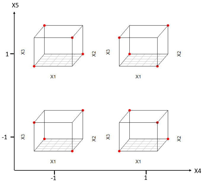
Figure 4.11: Resolution-5 design for five factors \(x_{1}-x_{5}\) depicted as five-dimensional trellis plot
| K | N.trials | Redundancy |
|---|---|---|
| 5 | 16 | 1.00 |
| 6 | 32 | 1.45 |
| 7 | 64 | 2.21 |
| 8 | 64 | 1.73 |
| 9 | 128 | 2.78 |
| 10 | 128 | 2.29 |
| 11 | 128 | 1.91 |
| 12 | 256 | 3.24 |
| 13 | 256 | 2.78 |
| 14 | 256 | 2.42 |
| 15 | 256 | 2.12 |
According to table 4.7 the relationship between R and K is not monotone anymore, so sometimes larger K leads to lower R(K) and higher dimensional designs can sometimes become more economical than lower dimensional designs in terms of R(K). However, the number of trials of resolution V designs grows rapidly simply by the fact that the number of two way interactions grows approximately quadratic with K according to \(\frac {K \cdot (K-1)}{2}\).
This again brings up the question whether further points of the full factorial designs can be omitted so as so render more parsimonious models estimable.
This is possible and will be demonstrated by constructing a 2(7-4) fractional factorial design from a 23 full factorial design. The construction process starts by fully expanding a 23 design as shown in table 4.8
| x1 | x2 | x3 | x1:x2 | x1:x3 | x2:x3 | x1:x2:x3 |
|---|---|---|---|---|---|---|
| -1 | -1 | -1 | 1 | 1 | 1 | -1 |
| 1 | -1 | -1 | -1 | -1 | 1 | 1 |
| -1 | 1 | -1 | -1 | 1 | -1 | 1 |
| 1 | 1 | -1 | 1 | -1 | -1 | -1 |
| -1 | -1 | 1 | 1 | -1 | -1 | 1 |
| 1 | -1 | 1 | -1 | 1 | -1 | -1 |
| -1 | 1 | 1 | -1 | -1 | 1 | -1 |
| 1 | 1 | 1 | 1 | 1 | 1 | 1 |
All interactions (in R notation) are know identified with new factor names according to
- x4 = x1:x2
- I = x1:x2:x4
- x5 = x1:x3
- I = x1:x3:x5
- x6 = x2:x3
- I = x2:x3:x6
- x7 = x1:x2:x3
- I = x1:x2:x3:x7
The shortest length of the defining contrasts in the list is three, hence the resolution of the thus constructed design is R=3. In this design all main effects are confounded with 2-way interactions or higher interactions and will be biased by these high order term (provided these terms are different from zero).
Fractional factorial resolution III designs belong to the class of screening designs and can be used for estimating the main effects of a large number of factors under the assumption that factor interactions can be neglected. With a 2(7-4) design seven main effects can be investigated with eight runs. The design is saturated and requires replicates at the design center for an estimate of the error variance.
In a similar way a 2(3-1) resolution III design can be constructed from a 22 factorial by the identity x3=x1:x2 and that allows estimating three main effects (x1,x2,x3) from four runs. This design and its complementary design are depicted in 4.12 with the complement being the part omitted from the full factorial design in creating the fractional factorials. Note that by combining a fractional factorial design with its complement, the original full factorials design is reconstructed.
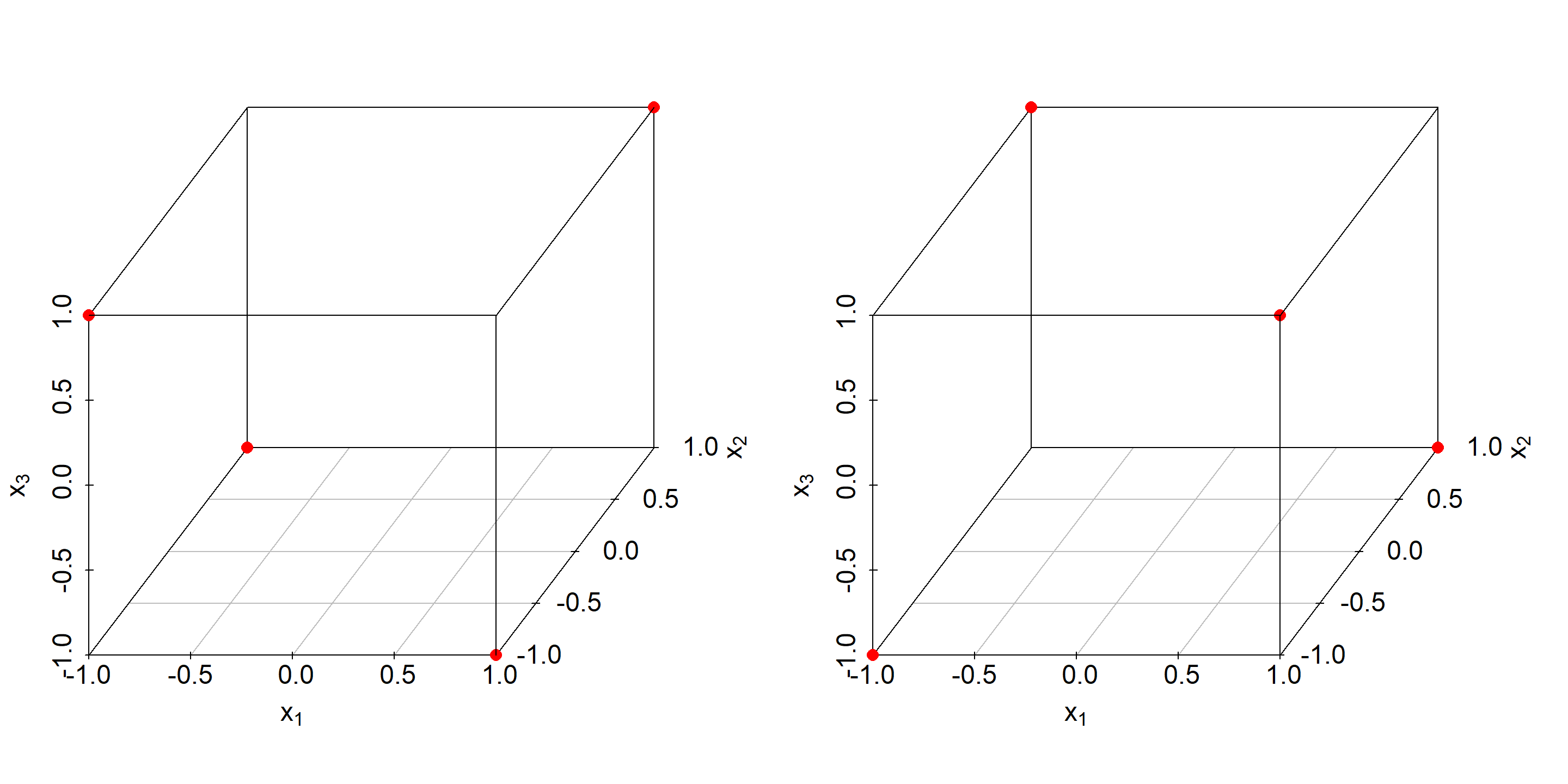
Figure 4.12: Fractional factorial resolution III design (left panel) and corresponding complementary design shown on the right panel.
Finally, a 2(4-1) fractional factorial resolution IV design will be derived from the expanded 23 design, table 4.8, by reassigning the 3-way contrast x1:x2:x3 to the factor x4. The defining contrast I = x1:x2:x3:x4 is of length 4, hence the designs is of resolution 4. In the so constructed resolution IV design, main effects are confonded with 3-way interactions (or higher), while 2-way interactions are confounded with 2-way interactions. Put differently, a resolution IV design can only identify a half fraction of the 2-way interactions with the other half being confounded. For the 2(4-1) resolution IV design it can be easily derived from the generator that the following three confounding conditions hold
- x1:x2=x3:x4
- x1:x3=x2:x4
- x1:x4=x2:x3
Resolution IV designs can play an important role in the sequential use of DoE. In experimental projects there is often uncertainty about the significance of interactions. In such a situation, it might be a good choice to estimate only a half fraction of the interaction terms in the first place. If, say, x1:x2 turns out significant in the outcome, the resolution IV design can be complemented easily to render the confounded pair x1:x2 and x3:x4 subsequentially estimable. Sequential strategies can reduce the experimental effort significantly. The FrF2 function aliasprint() reports the confounding structure of fractional factorial designs.
x <- FrF2::FrF2(nfactors=4,resolution=4,
    factor.names=paste("x",1:4,sep=""), ncenter=0, randomize=F)
FrF2::aliasprint(x)
## $legend
## [1] A=x1 B=x2 C=x3 D=x4
##
## $main
## character(0)
##
## $fi2
## [1] AB=CD AC=BD AD=BC4.5 Screening designs
When there are many potential factors, say K>8, of which only a small fraction can be assumed to exert large effects, screening design can be an option for identifying these high leverage candidates. As shown above, fractional factorial resolution III designs belong to the class of screening designs used for estimating K main effects with \(N \approx K\) runs. For instance, with the 2(7-4) resolution III design from above, we can screen the effects of seven parameters with 8 runs.
There is another class of non-regular fractional factorial screening designs, the Plackett-Burman designs (PB). The number of runs in a PB design is always a multiple of four as opposed to the fractional factorial designs, where the number of runs is always a multiple of two.
Table 4.9 gives an overview of available PB and resolution III designs for K=4, 5…19. It should be noted that PB and resolution III designs coincide for K=4,5,6,7. The list shows that factor number 11,15,19 all reveal redundancies of 1 for the PB designs making PB the design of choice for these factor number.
| K | N.PB | R.PB | N.FR3 | R.FR3 |
|---|---|---|---|---|
| 4 | 8 | 1.60 | 8 | 1.60 |
| 5 | 8 | 1.33 | 8 | 1.33 |
| 6 | 8 | 1.14 | 8 | 1.14 |
| 7 | 8 | 1.00 | 8 | 1.00 |
| 8 | 12 | 1.33 | 16 | 1.78 |
| 9 | 12 | 1.20 | 16 | 1.60 |
| 10 | 12 | 1.09 | 16 | 1.45 |
| 11 | 12 | 1.00 | 16 | 1.33 |
| 12 | 16 | 1.23 | 16 | 1.23 |
| 13 | 16 | 1.14 | 16 | 1.14 |
| 14 | 16 | 1.07 | 16 | 1.07 |
| 15 | 16 | 1.00 | 16 | 1.00 |
| 16 | 20 | 1.18 | 32 | 1.88 |
| 17 | 20 | 1.11 | 32 | 1.78 |
| 18 | 20 | 1.05 | 32 | 1.68 |
| 19 | 20 | 1.00 | 32 | 1.60 |
Recently (2011) a new class of screening designs was introduced by Jones and Nachtsheim, the Definite Screening Designs (DSD). DSDs are available for K=4-12 factors on three levels with a total of 2K+1 designs runs. DSDs have the property of not confounding main with square effects which can be useful when screening many potentially non-linear factors. The following R-code analyses the confounding properties of a DSD with K=5 by plotting the correlation matrix of all model terms up to second order in figure 4.13. There is virtually no correlation between the main effects and the square terms and the (exact) condition number \(\kappa=8.9\) naively suggests estimability of the full RSM model.
Caveat: Never use kappa on a model matrix with n.col>n.row! As already mentioned, \(\kappa\) measures closeness to singularity by requiring \(\lambda_{min}>0\) in \(\kappa = \frac {\lambda_{max}}{\lambda_{min}}\) and does not signal singularities from rank deficiency. In the present case with n.col(21)>n.row(11), there are ten zero eigenvalues35.
x <- daewr::DefScreen(m=5,c=0)
z <- model.matrix(~ (A + B + C + D + E)^2 +
                    I(A^2) + I(B^2)+ I(C^2)+ I(D^2)+ I(E^2) ,data=x)[,-1]
kappa(x.model  <- model.matrix(~ (A + B + C + D + E)^2 +
                                 I(A^2) + I(B^2)+ I(C^2)+
                                 I(D^2)+ I(E^2) ,data=data.frame(scale(x))),exact=T)
## [1] 8.85372dim(x.model)## [1] 11 21sv <- svd(x.model) # singular value decomposition
sv$d[1]/sv$d[length(sv$d)] # kappa from SVD## [1] 8.85372colnames(z) <- stringi::stri_replace_all_fixed(colnames(z),LETTERS[1:5],
paste("x",1:5,sep=""), vectorize_all = FALSE)
corrplot::corrplot(cor(z))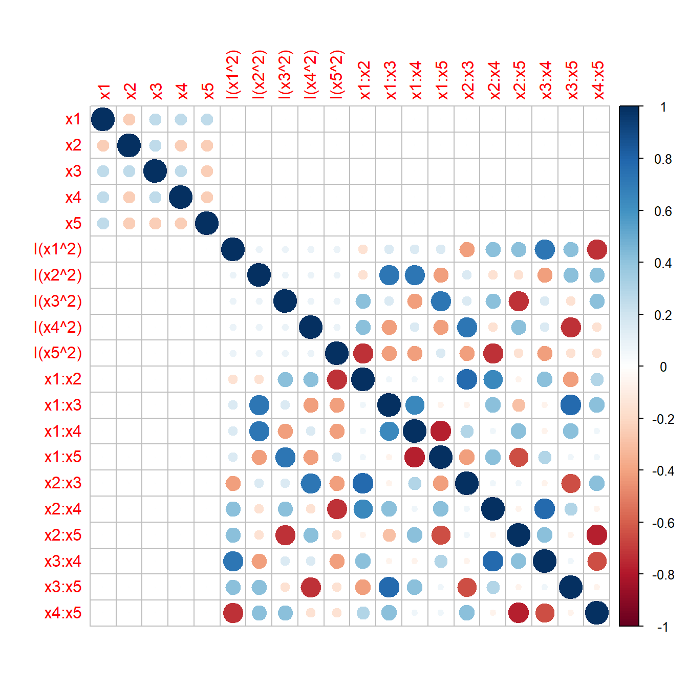
Figure 4.13: Pearson-r of all model terms up to second order of a Definite Screening Design for K=5
Despite this singularity, the power of DSDs for identifying non-linear effects under screening conditions (here 2K+1 rather than 1+2K+K(K-1)/2 design runs for RSM models) can be quite remarkable as the following simulation will demonstrate. A DSD for K=8 factors is created and a sample of the true model \(y=3x_{1} + 2x_{2} + x_{4} + x_{5} + 5x_{4} \cdot x_{5} + 3x_{3}^2 + 4x_{1}^2 + 2x_{6} + x_{7} + 5x_{7}^2 + \epsilon; \epsilon \sim N(0,1)\) is realized. The data is subsequently analyzed using a hierarchical step forward regression method from the library daewr with the user function step.forward(). It selects in a forward manner the terms maximizing the correlation between y and the partial residuals in a hierarchical model building process36. Model hierarchy is important as the significance of higher order terms can only be assessed with the lower order terms already present in the model. The results from eight forward steps are summarized in table 4.10 and the corresponding R2 values of each step are plotted in figure 4.14.
Results from eight forward, hierarchical RSM regression steps
## step.forward
## RSM forward regression keeping model hierarchy
##    y: Response vector
##    x: Data frame of x-variable
## step: Number of forward steps requested
## require(daewr)
rm(list=ls())
step.forward <- function(y,x,step)  {
  require(daewr)
  any.col       <- colnames(x)
  letter.col    <- LETTERS[1:ncol(x)]
  colnames(x)   <- letter.col
  xx            <- x
  xx$y          <- y

  cc <- sum(sapply(x,function(x) nlevels(as.factor(x)) ==2        ))
  mm <- sum(sapply(x,function(x) nlevels(as.factor(x)) ==3        ))


  suppressWarnings(invisible(capture.output(res<- ihstep(y,x,m=mm,c=cc)))    )
  f         <- paste("y~", paste(res,collapse="+"),sep="")
  f2        <- paste("y ~",paste(stringi::stri_replace_all_fixed(res,letter.col ,
                                                                 any.col, vectorize_all = FALSE),collapse="+"))
  collect   <- data.frame(formula=f2, R2= round(summary(lm(formula(f),data=xx) )$r.square,3)
                          ,stringsAsFactors = F     )

  for (i in (2:step)) {
    suppressWarnings( invisible(capture.output(res <- fhstep(y,x,m=mm,c=cc,res)))  )
    f          <- paste("y~", paste(res,collapse="+"),sep="")
    f2        <- paste("y ~",paste(stringi::stri_replace_all_fixed(res,letter.col ,
                                                                   any.col, vectorize_all = FALSE),collapse="+"))
    collect    <- rbind(collect,data.frame(formula=f2, R2= round(summary(lm(formula(f),data=xx) )$r.square,3),
                                           stringsAsFactors = F))
  }
  return(collect)
}
set.seed(1234)
x           <- daewr::DefScreen(m=8,c=0)
colnames(x) <- paste("x",1:8,sep="")
x$y         <-  3*x$x1 + 2*x$x2 + x$x4 + x$x5 +
  5*x$x4*x$x5 + 3*x$x3^2 +
  4*x$x1^2 + 2*x$x6 + x$x7 +
  5*x$x7^2 + rnorm(nrow(x),0,1)
z <- step.forward(x$y,x[,-9], 8 )
# show best model #4
summary(lm(formula(as.character(z[4,1])),data=x) )
##
## Call:
## lm(formula = formula(as.character(z[4, 1])), data = x)
##
## Residuals:
## Min 1Q Median 3Q Max
## -1.1103 -0.7592 -0.2003 0.6360 1.3022
##
## Coefficients:
## Estimate Std. Error t value Pr(>|t|)
## (Intercept) 0.5909 1.1303 0.523 0.619877
## I(x7^2) 5.1030 1.0770 4.738 0.003198 **
## x7 1.2834 0.3732 3.439 0.013824 *
## x2 2.0694 0.3732 5.545 0.001453 **
## x6 1.9827 0.3732 5.313 0.001808 **
## I(x1^2) 5.7737 1.0770 5.361 0.001727 **
## x1 2.9089 0.3732 7.794 0.000235 ***
## x4 1.2095 0.3732 3.241 0.017673 *
## x5 1.3971 0.3732 3.743 0.009583 **
## x2:x6 -0.7809 0.4937 -1.582 0.164816
## x4:x5 4.4906 0.4584 9.796 6.51e-05 ***
## ---
## Signif. codes: 0 '***' 0.001 '**' 0.01 '*' 0.05 '.' 0.1 ' ' 1
##
## Residual standard error: 1.396 on 6 degrees of freedom
## Multiple R-squared: 0.9875, Adjusted R-squared: 0.9666
## F-statistic: 47.24 on 10 and 6 DF, p-value: 6.647e-05z$formula <- gsub("^", "\\^", z$formula, fixed = T)
knitr::kable(
z, booktabs = TRUE, row.names=T,align="l",
caption = 'Results from eight forward,
hierarchical RSM regression steps
created from DSD data with the true model
$y=3x_{1} + 2x_{2} + x_{4} + x_{5} + 5x_{4} \\cdot x_{5} + 3x_{3}^2 + 4x_{1}^2 + 2x_{6} + x_{7} + 5x_{7}^2 + \\epsilon; \\epsilon \\sim N(0,1)$ ')| formula | R2 | |
|---|---|---|
| 1 | y ~ x4+x5+x4:x5 | 0.562 |
| 2 | y ~ I(x1^2)+x1+x4+x5+x4:x5 | 0.755 |
| 3 | y ~ x2+x6+x2:x6+I(x1^2)+x1+x4+x5+x4:x5 | 0.916 |
| 4 | y ~ I(x7^2)+x7+x2+x6+x2:x6+I(x1^2)+x1+x4+x5+x4:x5 | 0.987 |
| 5 | y ~ x2+x5+x2:x5+I(x7^2)+x7+x6+x2:x6+I(x1^2)+x1+x4+x4:x5 | 0.995 |
| 6 | y ~ x8+x2+x5+x2:x5+I(x7^2)+x7+x6+x2:x6+I(x1^2)+x1+x4+x4:x5 | 0.998 |
| 7 | y ~ x3+x8+x2+x5+x2:x5+I(x7^2)+x7+x6+x2:x6+I(x1^2)+x1+x4+x4:x5 | 1.000 |
| 8 | y ~ x5+x6+x5:x6+x3+x8+x2+x2:x5+I(x7^2)+x7+x2:x6+I(x1^2)+x1+x4+x4:x5 | 1.000 |
plot(1:nrow(z),z$R2,type="b", xlab="model index #",
     ylab=expression(paste("model R" ^ 2) ) )
grid()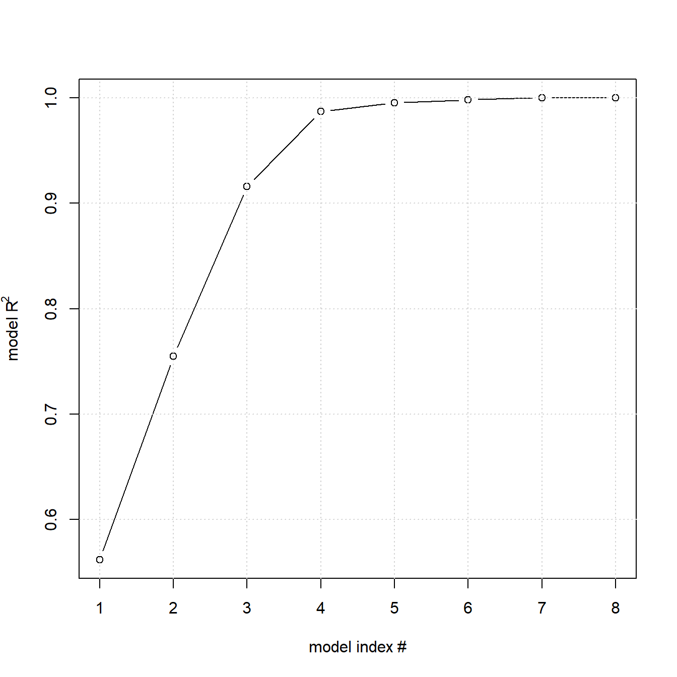
Figure 4.14: Results from eight forward, hierarchical RSM regression steps with the true model \(y=3x_{1} + 2x_{2} + x_{4} + x_{5} + 5x_{4} \cdot x_{5} + 3x_{3}^2 + 4x_{1}^2 + 2x_{6} + x_{7} + 5x_{7}^2 + \epsilon; \epsilon \sim N(0,1)\)
The marked shoulder of model #4 in figure 4.14 recommends this model as local solution, and this model correctly identifies nine out of ten model terms unbiasedly (the term x2:x6 was erroneously selected, the term x32 was missed). This result clearly shows that DSDs should be an option when dealing with many, potentially non-linear factors in a screening situation.
4.6 Response surface model designs (RSM designs)
RSM designs aim at identifying all model terms in a full 2nd order model of the general parametric form \[f(\Delta x_{1}, \Delta x_{2}... \Delta x_{I}) \approx a_{0} + \sum_{i}a_{i}\cdot \Delta x_{i} + \sum_{i}a_{ii}\cdot \Delta x_{i}^2 + \sum_{j>i}a_{ij}\cdot \Delta x_{i}\cdot \Delta x_{j}\] Central Composite (CC) designs are a versatile and flexibel class of designs of first choice for optimally identifying response surface models. As the name already suggests, they are a composite of a factorial (or fractional factorial) part and a so called star part. The CC designs come in two subclasses, namely the Central Composite-Circumscribed (CCC) designs and the Central Composite-Face centered (CCF) designs. Figure 4.15 shows examples of CCC and CCF designs in \(\mathbb{R^3}\) with the factorial and star part labelled red and blue, respectively. In the CCC designs the stars protrude beyond the cube faces, while in a CCF design the star points lie on the cube surface. Consequently, in a CCC design the factors are on five levels, namely and in coded units: \(-\alpha,-1,0,1,\alpha\), while in a CCF designs the factors are on three levels only, that is -1,0,1. Logistically, CCF designs are easier to handle in the laboratory at the expense of having somewhat lower statistical properties compared to CCC designs.
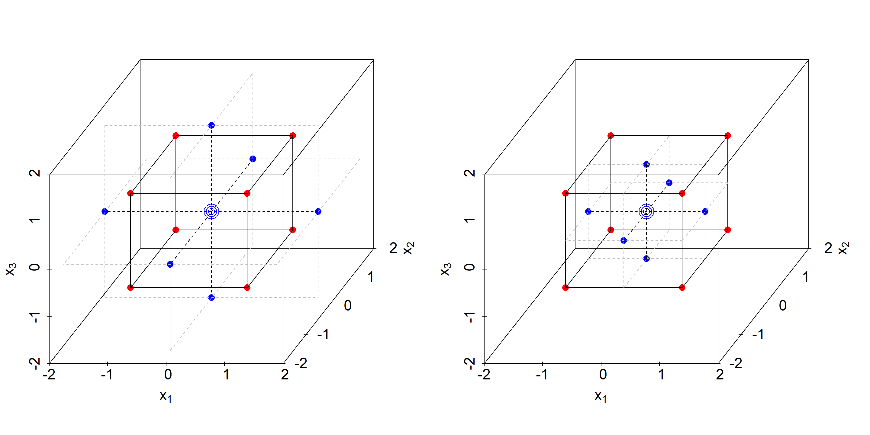
Figure 4.15: Central-Composite-Circumscribed (CCC, left panel) and Central-Composite Face-centered (CCF, right panel) designs for K=3 in coded units
The extension of the star part \(\alpha\) affects the statistical properties of the CCC designs. For a rotateable CCC design with Nfac points in the factorial part, \(\alpha\) is simply given by the expression \(\alpha_{rotateable}=\sqrt[4] {N_{fac}}\) which will render the variance function equal ([hyper]spherical) in all direction of experimental space. Alternatively, \(\alpha\) can be choosen to make the star and factorial part orthogonal, i.e. is a block variable labelling both parts with {0,1} will be maximal unconfounded with the RSM model parameters. This property can be important when using CC designs sequentially by starting with a factorial design first and augmenting the factorial part by star points later. The following R-code shows a typical analysis of a RSM design using functions from the library “rsm” and the library “lattice”.
rm(list=ls())
library(lattice)
set.seed(123)
x             <- data.frame(rsm::ccd(3,alpha="orthogonal",randomize=F,
                  n0=c(3,0)))[,-c(1,2)]
colnames(x)   <- c(paste("x",1:3,sep=""),"Block")
x             <- x[order(runif(nrow(x))),]
rownames(x)   <- NULL
knitr::kable(
  x, booktabs = TRUE,row.names=T, digits=3,align="c",
  caption = 'CCC design with 3 center points and
orthogonal blocking')| x1 | x2 | x3 | Block | |
|---|---|---|---|---|
| 1 | 1.000 | -1.000 | 1.000 | 1 |
| 2 | 0.000 | 1.477 | 0.000 | 2 |
| 3 | 0.000 | 0.000 | 1.477 | 2 |
| 4 | -1.000 | -1.000 | -1.000 | 1 |
| 5 | -1.000 | 1.000 | -1.000 | 1 |
| 6 | -1.477 | 0.000 | 0.000 | 2 |
| 7 | 0.000 | 0.000 | 0.000 | 1 |
| 8 | -1.000 | 1.000 | 1.000 | 1 |
| 9 | 0.000 | 0.000 | 0.000 | 1 |
| 10 | 0.000 | -1.477 | 0.000 | 2 |
| 11 | 1.477 | 0.000 | 0.000 | 2 |
| 12 | 1.000 | -1.000 | -1.000 | 1 |
| 13 | 1.000 | 1.000 | -1.000 | 1 |
| 14 | 1.000 | 1.000 | 1.000 | 1 |
| 15 | 0.000 | 0.000 | -1.477 | 2 |
| 16 | -1.000 | -1.000 | 1.000 | 1 |
| 17 | 0.000 | 0.000 | 0.000 | 1 |
x$y <- 20*(x$Block==2)  + 3*x$x1 + 5*x$x2 +
  6*x$x3 + 5*x$x1^2 + 8*x$x2^2 + 5*x$x3^2 + rnorm(nrow(x),0,1)
              # Block=0: factorial; Block=1:star
summary(res <- rsm::rsm(y~Block + SO(x1,x2,x3), data=x))
##
## Call:
## rsm(formula = y ~ Block + SO(x1, x2, x3), data = x)
##
## Estimate Std. Error t value Pr(>|t|)
## (Intercept) 0.28242 0.63342 0.4459 0.6713339
## Block2 19.89145 0.55681 35.7241 3.208e-08 ***
## x1 2.28752 0.31202 7.3314 0.0003291 ***
## x2 5.31461 0.31202 17.0330 2.619e-06 ***
## x3 5.94880 0.31202 19.0656 1.346e-06 ***
## x1:x2 0.31363 0.38789 0.8086 0.4496323
## x1:x3 0.09441 0.38789 0.2434 0.8158084
## x2:x3 0.52927 0.38789 1.3645 0.2213735
## x1^2 4.79514 0.38155 12.5675 1.553e-05 ***
## x2^2 8.29488 0.38155 21.7398 6.186e-07 ***
## x3^2 4.78696 0.38155 12.5460 1.569e-05 ***
## ---
## Signif. codes: 0 '***' 0.001 '**' 0.01 '*' 0.05 '.' 0.1 ' ' 1
##
## Multiple R-squared: 0.9977, Adjusted R-squared: 0.9939
## F-statistic: 263 on 10 and 6 DF, p-value: 4.098e-07
##
## Analysis of Variance Table
##
## Response: y
## Df Sum Sq Mean Sq F value Pr(>F)
## Block 1 1536.13 1536.13 1276.2107 3.208e-08
## FO(x1, x2, x3) 3 851.44 283.81 235.7896 1.297e-06
## TWI(x1, x2, x3) 3 3.10 1.03 0.8583 0.5117
## PQ(x1, x2, x3) 3 775.20 258.40 214.6783 1.714e-06
## Residuals 6 7.22 1.20
## Lack of fit 4 4.53 1.13 0.8431 0.6060
## Pure error 2 2.69 1.34
##
## Stationary point of response surface:
## x1 x2 x3
## -0.2228815 -0.2969119 -0.6027428
##
## Eigenanalysis:
## eigen() decomposition
## $values
## [1] 8.321983 4.814304 4.740696
##
## $vectors
## [,1] [,2] [,3]
## x1 -0.04529810 0.79991654 -0.59839921
## x2 -0.99614083 -0.08124721 -0.03320141
## x3 -0.07517663 0.59458592 0.80050987# RSM plot within rsm
#par(mfrow=c(1,2))
#persp(res,~x1+x2,at=list(x3=-1.477098),zlab="y",zlim=c(-15,60))
#persp(res,~x1+x2,at=list(x3=1.477098),zlab="y",zlim=c(-15,60))
# rsm plot trellis plot with lattice
x.pred <- expand.grid(x1 = seq( -1.477098, 1.477098, length=15),
x2 = seq(-1.477098, 1.477098, length=15),
x3 = seq(-1.477098, 1.477098, length=3),
Block = c(1,2) )
x.pred$Block <- factor(x.pred$Block)
x.pred$y1 <- predict(res,x.pred)
wireframe(y1 ~ x1*x2|x3*Block, data=x.pred,
zlab=list(label="y",cex=1,rot=90),
xlab=list(label=expression(x [1]),cex=1,rot=0),
ylab=list(label=expression(x [2]),cex=1,rot=0),
zlim=c(-10,80),
drape=TRUE,
at=lattice::do.breaks(c(-10,80),100),
col.regions = pals::parula(100),
par.strip.text=list(cex=1.5),
strip=strip.custom(var.name=expression(x [3])),
scales = list(arrows = FALSE,
x=c(cex=1),
y=c(cex=1),
z=c(cex=1)) ,
screen = list(z = 60, x = -55, y=0)) 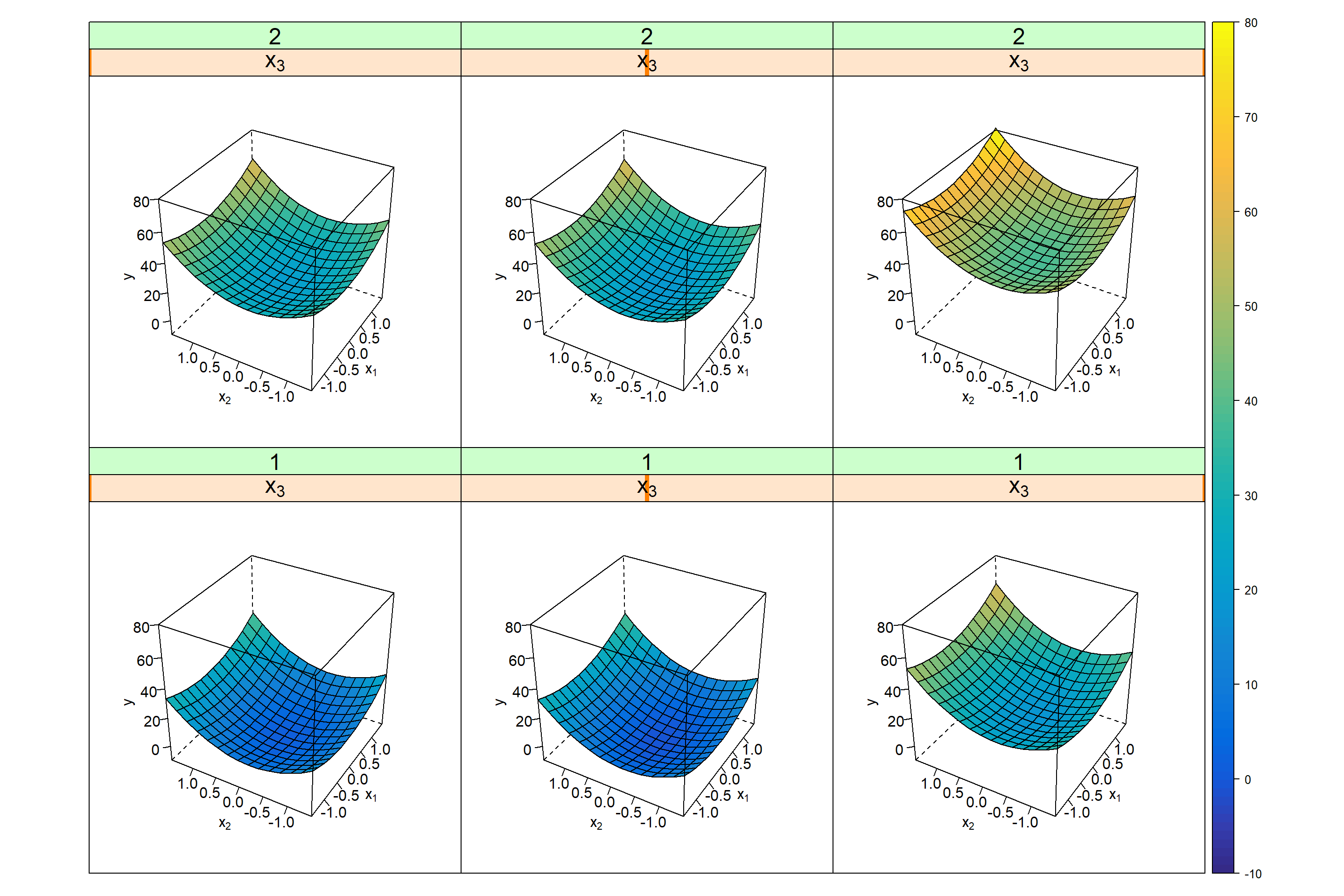
Figure 4.16: RSM trellis plot \(\hat y = f(x_{1},x_{2},x_{3},Block)\) including block effect Block=1(labelling the factorial part) and Block=2(corresponding to the star part). The variable Block is on the outer y-axis (on two levels 1,2), x3 on the outer x-axis, and x1 and x2 are on the inner x- and y-axes.
In addition to the known OLS results, the rsm function reports stationary points (max, min or sattle point). The nature of the stationary point is indicated by the eigenvalues \(\lambda_{i}\) in the output section “eigenanalysis” with \(\lambda_{i}>0 \ \forall i \rightarrow min; \lambda_{i}<0 \ \forall i \rightarrow max; \ else \ sattle\). In the present case all eigenvalues are strictly positive thus indicating a minimum that is reported at \(x_{1}^*=-0.332;\ x_{2}^*=-0.361;\ x_{3}^*=-0.696\). Furthermore, the function rsm decomposes the response variance into five contributing terms, namely
- Variance contribution (VC) of the block variable Block
- VC arising from the linear terms (abreviated FO(…))
- VC from bilinear interactions, TWI(…)
- VC from square terms, PQ(…)
- VC of the error term, the residuals, with the residual term further decomposed into
- Lack of Fit
- Pure Error
F-test results reveal no evidence of interactions or lack of fit and the replicates at the center are correctly predicted by the model within the replication (or pure) error. Lack of Fit, e.g., may result from systematic shifts between factorial and star points and can be accommodated by including a block variable as shown in the example above (rerunning the analysis with Block excluded leads to biased estimates indicated by pLoF=0.00048). The topology of the response surface can be visualized by plotting the model predictions over a grid of points with conditional 3D plots (trellis plots) y~f(x1,x2)|x3,x4 with x3 and x4 on the outer axes.
Figure 4.16 depicts the model y=f(x1,x2,x3,Block) as a 5D-trellis plot with two inner axes x1,x2 and two outer x-axes x3 and Block. The trellis plot reveals a minimum close to the center (0,0,0) with the exact location of the minimum in the plot remaining somewhat vague. Here, rsm helps by reporting the numerical solution of the minimum, \(x_{1}^*=-0.223;\ x_{2}^*=-0.297;\ x_{3}^*=-0.603\).
As the list of available CC design shows, see table 4.12, the design size N=f(K) grows large rapidly with dimension K, prohibiting the use of CC designs with K>4 in a normal lab (low-throughput) setup.
| K | N | orthogonal | rotateable | R |
|---|---|---|---|---|
| 2 | 11 | 1.069 | 1.414 | 1.83 |
| 3 | 17 | 1.477 | 1.682 | 1.70 |
| 4 | 27 | 1.835 | 2.000 | 1.80 |
| 5 | 45 | 2.138 | 2.378 | 2.14 |
| 6 | 79 | 2.394 | 2.828 | 2.82 |
| 7 | 145 | 2.615 | 3.364 | 4.03 |
Box-Behnken designs (BBD) as a class of reduced 33 designs are a parsimonious alternative to CC designs for estimating quadratic models. Table 4.13 lists the available designs and figure 4.17 shows a Box-Behnken design in three dimensions. Comparision of table 4.13 with 4.12 shows that CC and Box-Behnken designs are complementary in terms of model redundancy, and economical RSM designs may be found with the selection criterion min(RBBD, RCC).
| K | N | R |
|---|---|---|
| 3 | 15 | 1.50 |
| 4 | 33 | 2.20 |
| 5 | 46 | 2.19 |
| 6 | 51 | 1.82 |
| 7 | 59 | 1.64 |
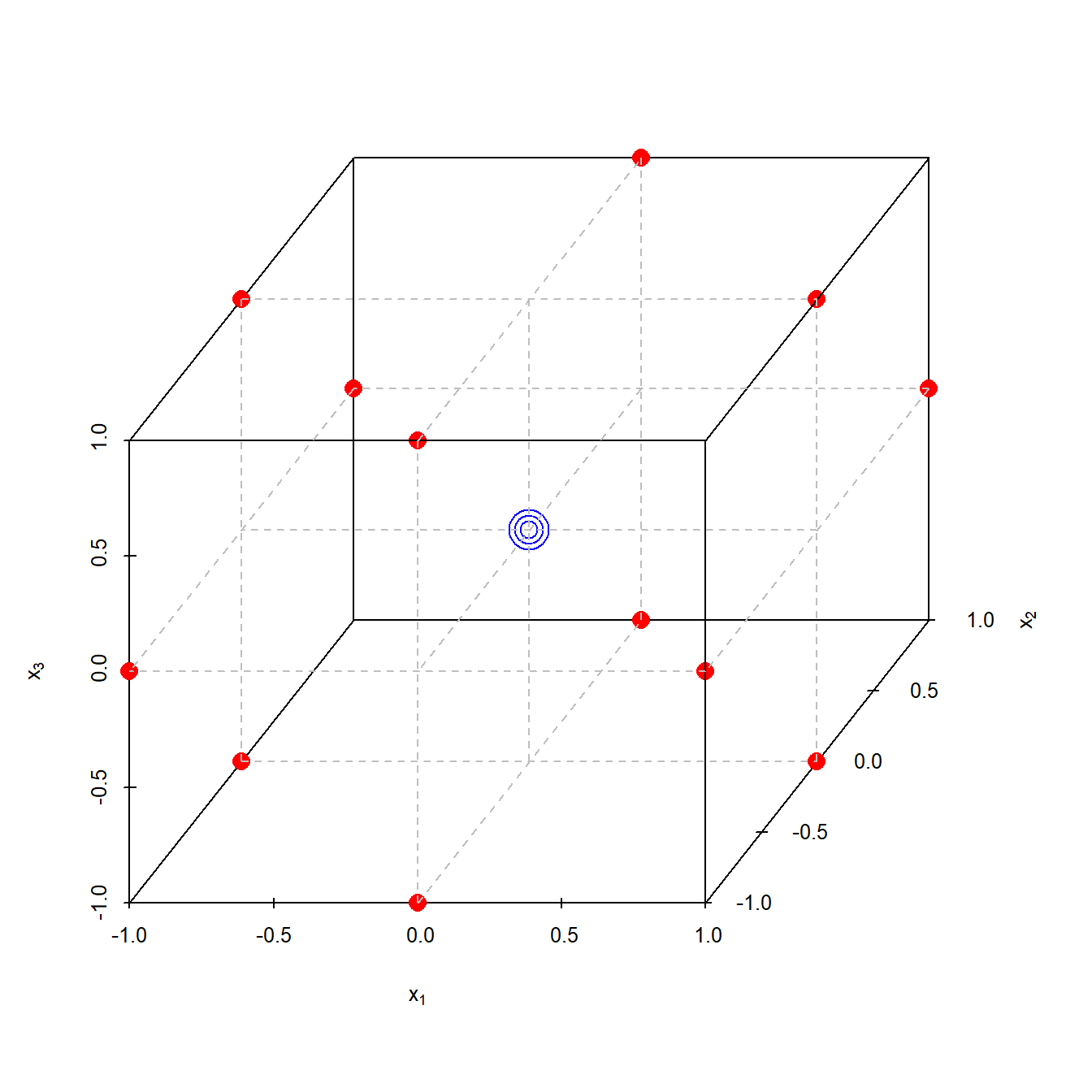
Figure 4.17: Three dimensional coded Box-Behnken design with three center points
4.7 Optimal designs
The designs discussed so far are classical designs, i.e. given complexity - linear, bilinear or quadratic - and dimensionality K the number of design runs and the parametric model are fixed and set by the design class. A fractional factorial resolution V design, as an example, will always support all bilinear models terms with a fixed number of runs irrespective of whether all interactions are physically possible.
Different from the classical designs, optimal or computer algorithmic designs define a more flexible class of designs able to handle almost all sort of experimental constraints, namely
- Any linear model can be specified by the user, for instance a three factor design x1,x2,x3 with only one possible interaction can be specified in R-notation by ~ x1+x2+x3+x1:x2.
- Any number of design runs with R(K)>1 can be specified allowing flexible and parsimonious experimentation.
- Complex constraints can be handled by excluding infeasible runs and regions from the candidate set prior to design generation.
- Existing data can be augmented to render a parametric model estimable in a process similar to augmenting a factorial design by star points. However, optimal augmentation does nor require the data to be of factorial and fractional factorial nature. In principle, any non-singular data set, historical or from DoE, can be augmented.
Optimal designs are created from a set of potential candidate points, typically 3K full factorial designs (or higher). When there are constraints, they are applied to the candidate set (often linear constraints such as \(LB_{i} \leq \sum_{i}a_{i} \cdot x_{i} \leq UB_{i}\)) and, given model and number of desired runs, the optimal design is obtained by optimally selecting designs points from the candidate set using an alphabetic optimization objective. There are many scalar objective functions available, such as A-, G- or D-optimality to name but a few with the latter, D-optimality, being the most common seeking to minimize the determinant (indicated by |.|) of the inverse information matrix, i.e. \[{\min_{X} |(\boldsymbol {X^{T}X)^{-1}}}|\] A visual overview of the process of generating optimal (constrained and unconstrained) designs from a list of candidate points is depicted in figure 4.18.
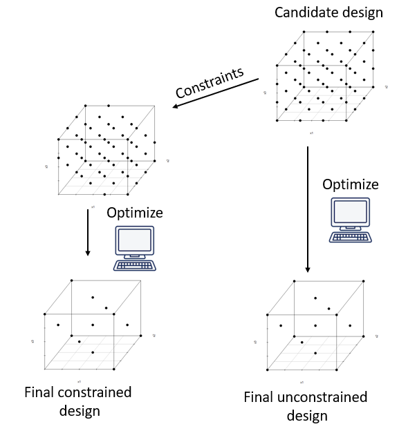
Figure 4.18: Process of generating an optimal designs from a set of candidate points
It should be noted that optimal designs are not necessarily superiour to classical design as the following example will show. The example code juxtaposes a classical CCF design of size N=17 with a D-optimal RSM design of the same size, see figure 4.19, and reports some design criteria, namely
- CCF design: \(\kappa=3.03\), D-optimality=0.413
- D-optimal design: \(\kappa=4.03\), D-optimality=0.458
The CCF design is better than the D-optimal design both in terms of \(\kappa\) and D-criteria. Figure 4.19 reveals the poor balance of the D-optimal design compared to the CCF design with the consequence being that the accuracy of the design becomes dependent on the direction in experimental space. Generating optimal designs is computationally difficult as there are many local minima of the objective function and, as the example showed, there is no guarantee that the optimizer will find the global optimum (the CCF design in the example).
rm(list=ls())
candidate <- expand.grid(x1=c(-1,0,1),  # 3^3 candidate design
                         x2=c(-1,0,1),
                         x3=c(-1,0,1) )
set.seed(1234)
doe <- AlgDesign::optFederov(~ (x1+x2+x3)^2+
                               I(x1^2) + I(x2^2) + I(x3^2),
                      data=candidate,center=T,
                      criterion="D", nTrials=17)$design
                      # d-optimal design with 17 runs
kappa(model.matrix(~ (x1+x2+x3)^2+ I(x1^2) +
            I(x2^2) + I(x3^2), data=doe)) # kappa doe
## [1] 4.02569kappa(model.matrix(~ (x1+x2+x3)^2+ I(x1^2)
+ I(x2^2) + I(x3^2),
data=rsm::ccd(3, n0=c(3,0),
randomize=F,alpha=1)[,3:5])) # kappa CCF design## [1] 3.025454AlgDesign::eval.design(~ (x1+x2+x3)^2+ I(x1^2)
+ I(x2^2) + I(x3^2),doe) # D=0.4583859 ## $determinant
## [1] 0.4583859
##
## $A
## [1] 3.751222
##
## $diagonality
## [1] 0.78
##
## $gmean.variances
## [1] 2.436736AlgDesign::eval.design(~ (x1+x2+x3)^2+
I(x1^2) + I(x2^2) + I(x3^2),
rsm::ccd(3, n0=c(3,0), randomize=F
,alpha=1)[,3:5]) # D=0.4129647## $determinant
## [1] 0.4129647
##
## $A
## [1] 3.362289
##
## $diagonality
## [1] 0.778
##
## $gmean.variances
## [1] 2.840631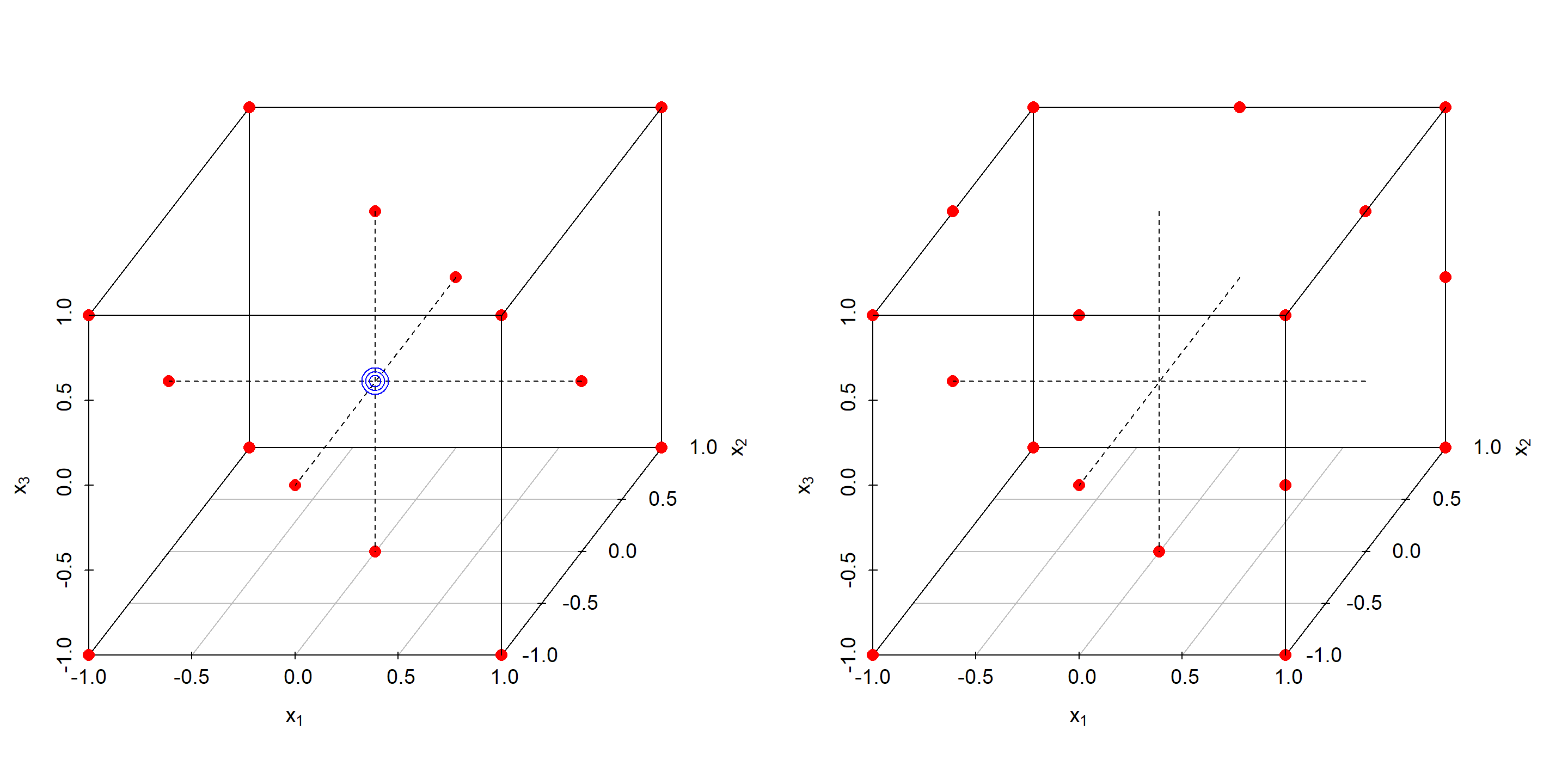
Figure 4.19: CCF design with three center points and N=17 (left panel) compared to D-optimal RSM design with 17 runs (right panel)
The difference in model accuracy can be visualized with the variance dispersion graph (with the R function Vdgraph::Vdgraph(…)) shown in figure 4.20, depicting the average model variance as a function of the coded design radius. Direction dependence is indicated by the upper and lower limits of the variance (note that for a rotateable CCC design max, min and average variance coincide).
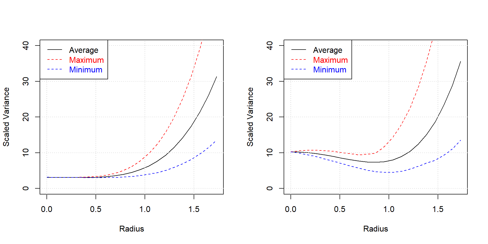
Figure 4.20: Variance dispersion graphs for the K=3, N=17, CCF design (left panel) compared with the K=3, N=17 D-optimal design (right panel)
Model accuracy as a function of the radius is better for the CCF design compared with the D-optimal design as expected. However, this “lack of optimality” of optimal designs is often outweighted by their higher flexibility and there are practitioner exclusively working with these designs, something not recommended here. Whenever possible, classical designs are to be preferred over optimal designs for their better statistical properties.
The following example is a typical application of an optimal design and borrowed from chapter 7. In an optimization project aiming at maximizing catalytic performance ton.dmm over a set of 7 influential factors, a subspace comprising 9 runs was identify from a historical record with the condition ton.dmm>400. In this subset T, p.h2, p.co2 and t.h were found constant at T=90, p.h2=90, p.co2=20 and t.h=18 thereby suggesting to conditionally optimze m.kat, v.ml and m.add first while keeping the remaining 4 variables constant at T=90, p.h2=90, p.co2=20 and t.h=18 for the time being. A full factorial 3x3x3 (33) design was created as a set of candidate points and the nine runs from the historical data were augmented by another set of six runs optimally selected from the candidate set so as to render a full second order design of the factors m.kat, v.ml, m.add estimable. The following R-code does the augmentation and plots the augmented data set.
rm(list=ls())
m.kat <- scan(text=" 0.18750  0.3750  0.750  0.3750  0.375
              0.375  0.3750  0.375  0.3750")
v.ml  <- scan(text="0.50000  0.5000  0.500  0.5000  0.500
              0.500  0.5000  0.500  0.2500")
m.add <- scan(text=" 0.78125  1.5625  3.125  0.9375  1.250
              1.875  2.1875  2.500  1.5625")
T     <- scan(text="90.00000 90.0000 90.000 90.0000 90.000
              90.000 90.0000 90.000 90.0000")
p.h2  <- scan(text="90.00000 90.0000 90.000 90.0000 90.000
              90.000 90.0000 90.000 90.0000")
p.co2 <- scan(text="20.00000 20.0000 20.000 20.0000 20.000
              20.000 20.0000 20.000 20.0000")
t.h   <- scan(text="18.00000 18.0000 18.000 18.0000 18.000
              18.000 18.0000 18.000 18.0000")

x.promising <- data.frame(m.kat, v.ml, m.add, T,p.h2, p.co2, t.h)

sapply(x.promising,range) # report ranges
## m.kat v.ml m.add T p.h2 p.co2 t.h
## [1,] 0.1875 0.25 0.78125 90 90 20 18
## [2,] 0.7500 0.50 3.12500 90 90 20 18round(cor(x.promising[,1:3]),2) # ...and Pearson r## m.kat v.ml m.add
## m.kat 1.00 0.05 0.79
## v.ml 0.05 1.00 0.09
## m.add 0.79 0.09 1.00candidate <- expand.grid(m.kat=seq(min(x.promising$m.kat),
max(x.promising$m.kat),length=3),
v.ml=seq(min(x.promising$v.ml),
max(x.promising$v.ml) ,length=3),
m.add=seq(min(x.promising$m.add),
max(x.promising$m.add),length=3) )
candidate <- rbind(x.promising[,1:3],candidate)
# rowbind x.promising and candidate set
kappa(model.matrix(~ (m.kat + v.ml + m.add)^2 +
I(m.kat^2) + I(v.ml^2) + I(m.add^2) ,
data=data.frame(scale(x.promising) ) ) )## [1] 3.863113e+17set.seed(12345)
doe.cat <- AlgDesign::optFederov(~ (m.kat + v.ml + m.add)^2+
I(m.kat^2) + I(v.ml^2) + I(m.add^2),
data=candidate,center=T,augment=T,rows=(1:9),
criterion="D", nTrials=15)$design
# d-optimal cat design
# comprising 9 historical
# and 6 additional candidates from candidate set
rownames(doe.cat ) <- NULL
kappa(model.matrix(~ (m.kat + v.ml + m.add)^2 +
I(m.kat^2) + I(v.ml^2) + I(m.add^2) ,
data=data.frame(scale(doe.cat) ) ) )## [1] 8.519979round(cor(doe.cat),2)## m.kat v.ml m.add
## m.kat 1.00 -0.20 0.07
## v.ml -0.20 1.00 -0.27
## m.add 0.07 -0.27 1.00s3d <- scatterplot3d::scatterplot3d(doe.cat, type="p",
highlight.3d=F,tick.marks=T,xlab="m.kat",
ylab="v.ml",zlab="m.add",
angle=55, scale.y=1, pch=16 ,
color=c(rep("red",9), rep("blue",6)) ,
cex.symbol=1.5, cex.lab = 0.8 )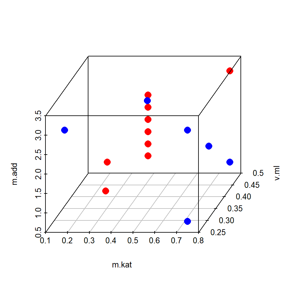
Figure 4.21: Historical trials m.kat, v.ml, m.add (red) augmented by six augmentation trials (blue)
Note how the comparatively large correlation between m.kat and m.add (rm.add,m.kat=0.79) prior to augmentation is counterbalanced by the augmentation trials into rm.add,m.kat=0.07. All effects up to 2nd order, which were formerly non-estimable in the historical data, are now estimable with the augmented data (\(\kappa=8.5\)). Figure 4.21 shows the historical core design (labelled red) along with the augmentation trials (labelled blue).
4.7.1 Example on the sequential use of RSM designs
CC and optimal designs both offer the possibility to build up models sequentially by starting with designs of low complexity which will then be gradually augmented to render more complex models estimable if indications of higher order effects arise in the course of the project. The data of the following example is taken from (George E.P. Box, Norman R. Draper 1987) pp. 306-322, and the aim of the project was finding conditions maximizing the elasticity of a polymer blend37. Three influential factors were identified by the practitioners with the following initial ranges
- Concentration of the first component conc1 [%] = {15,21}
- Concentration of the second component conc2 [%] = {2.3,3.1}
- Temperature Temp [o C] = {135,155}
A 23 full factorial design without center points was set-up straddling the “so far best conditions” derived from previous experiments. There are many ways of creating a 23 design in R, here the library rsm is used as the package supports sequential buildup of CC designs from factorial designs. The designs are specified in coded variables, here abbreviated x1,x2,x3, from which the uncoded variables were obtained by the linear transformation \(var_{coded}=\frac {var_{uncoded} - center} {midrange}\).
rm(list=ls())
set.seed(12345)
fac <-rsm::cube(~x1+x2+x3,n0=0, randomize=TRUE,
coding=list(x1~ (conc1-18)/3 ,x2~(conc2-2.7)/0.4,
            x3~(Temp-145)/10))
fac
## run.order std.order conc1 conc2 Temp
## 1 1 6 21 2.3 155
## 2 2 5 15 2.3 155
## 3 3 7 15 3.1 155
## 4 4 8 21 3.1 155
## 5 5 3 15 3.1 135
## 6 6 1 15 2.3 135
## 7 7 2 21 2.3 135
## 8 8 4 21 3.1 135
##
## Data are stored in coded form using these coding formulas ...
## x1 ~ (conc1 - 18)/3
## x2 ~ (conc2 - 2.7)/0.4
## x3 ~ (Temp - 145)/10The data is internally stored in coded units, however uncoded variables are printed to be performed in the laboratory in randomized order. The factorial results were analysed with the rsm() function and visualized with a trellis response surface plot.
rm(list=ls())
conc1 <- scan(text="15  21  15  21  15  21  15  21")
conc2 <- scan(text="2.3 2.3 3.1 3.1 2.3 2.3 3.1 3.1")
Temp <- scan(text="135  135 135 135 155 155 155 155")
y    <- scan(text="25.74    48.98   42.78   35.94   41.5
             50.1   46.06   27.7")
x <- data.frame(conc1,conc2,Temp,y)
summary(res <- rsm::rsm(y~FO(conc1,conc2,Temp)+
                          TWI(conc1,conc2,Temp) , data=x))
##
## Call:
## rsm(formula = y ~ FO(conc1, conc2, Temp) + TWI(conc1, conc2,
## Temp), data = x)
##
## Estimate Std. Error t value Pr(>|t|)
## (Intercept) -815.51125 53.87307 -15.1376 0.04199 *
## conc1 32.12417 2.08330 15.4199 0.04123 *
## conc2 201.58750 15.33108 13.1489 0.04832 *
## Temp 3.95375 0.35437 11.1571 0.05691 .
## conc1:conc2 -5.94167 0.32500 -18.2821 0.03479 *
## conc1:Temp -0.10900 0.01300 -8.3846 0.07557 .
## conc2:Temp -0.68250 0.09750 -7.0000 0.09033 .
## ---
## Signif. codes: 0 '***' 0.001 '**' 0.01 '*' 0.05 '.' 0.1 ' ' 1
##
## Multiple R-squared: 0.998, Adjusted R-squared: 0.9858
## F-statistic: 82.06 on 6 and 1 DF, p-value: 0.0843
##
## Analysis of Variance Table
##
## Response: y
## Df Sum Sq Mean Sq F value Pr(>F)
## FO(conc1, conc2, Temp) 3 47.22 15.738 12.934 0.2010
## TWI(conc1, conc2, Temp) 3 551.86 183.954 151.178 0.0597
## Residuals 1 1.22 1.217
## Lack of fit 1 1.22 1.217
## Pure error 0 0.00
##
## Stationary point of response surface:
## conc1 conc2 Temp
## 18.173752 2.890566 137.150362
##
## Eigenanalysis:
## eigen() decomposition
## $values
## [1] 2.98466894 0.01235354 -2.99702248
##
## $vectors
## [,1] [,2] [,3]
## conc1 0.70320084 -0.11402556 -0.70178825
## conc2 -0.70772462 -0.01774831 -0.70626543
## Temp 0.06807676 0.99331927 -0.09317933x.pred <- expand.grid(conc1 = seq( min(x$conc1),
max(x$conc1), length=15),
conc2 = seq( min(x$conc2),
max(x$conc2), length=15),
Temp = seq( min(x$Temp),
max(x$Temp), length=3) )
x.pred$y <- predict(res,x.pred)
lattice::wireframe(y~conc1*conc2|Temp, data=x.pred,layout=c(3,1),
zlab=list(label="y",cex=1.3,rot=90),
xlab=list(label=expression(conc [1]),cex=1.3,rot=55),
ylab=list(label=expression(conc [2]),cex=1.3,rot=0),
drape=TRUE,
par.strip.text=list(cex=1.5),
col.regions = pals::parula(100),
strip=T,
scales = list(arrows = FALSE,
x=c(cex=1.3),
y=c(cex=1.3),
z=c(cex=1.3)) ,
screen = list(z = 60, x = -55, y=0)) 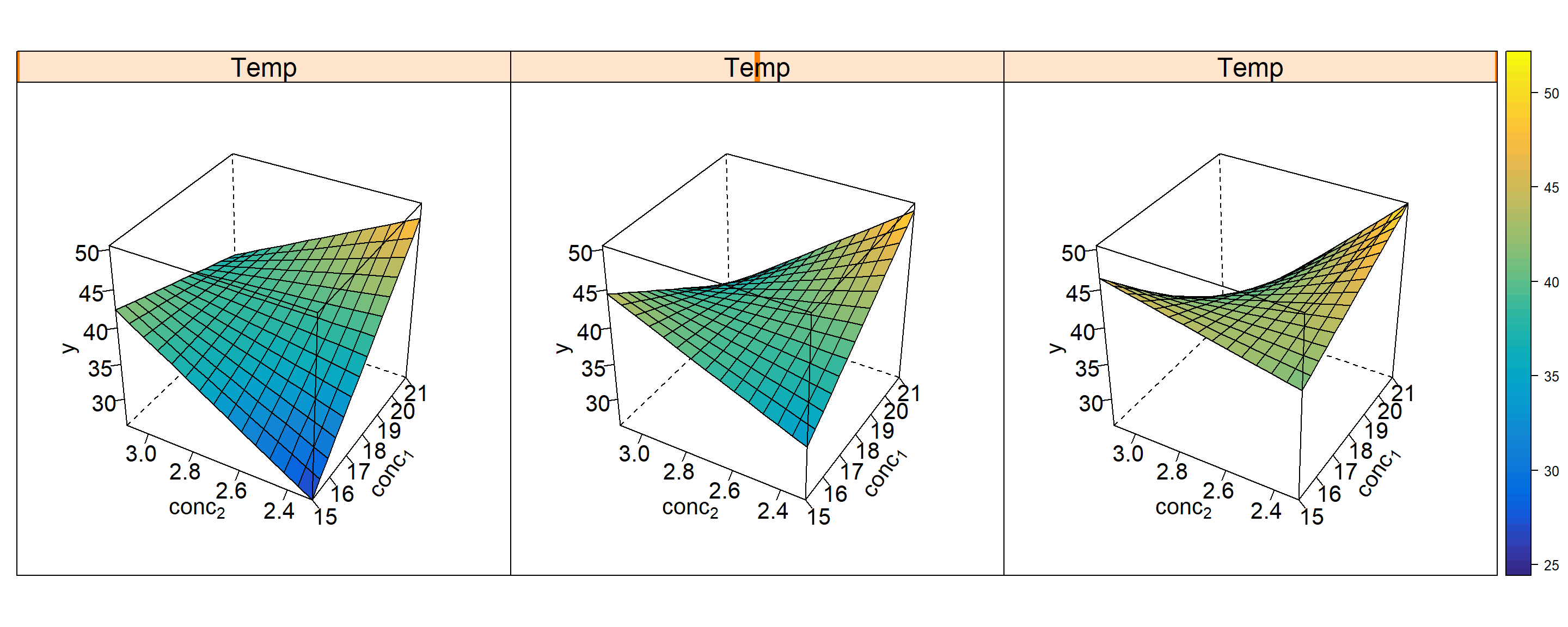
Figure 4.22: Response Surface trellis plot \(\hat y=f(conc_{1},conc_{2},Temp)\) of factorial polymer elasticity \(\hat y\)
The trellis plots, figure 4.22, as well as rsm-output show, that the system is dominated by interactions. In the rsm-output for example, interactions TWI() explain a large portion, SS=552, of the variance compared with minor linear contributions FO(), SS=47, and, as a consequence, the response surface trellis plot resembles a twisted plain. Given this nonlinear topology and lacking center point(!), it would be dangerous to take the suggested path of further ascend in figure 4.22 seriously, namely increase Temp and conc1 while decreasing conc2. It seems more reasonable to suspect that there are strong nonlinear effects underlying the system which the bilinear model (data) cannot appropriately describe.
This was also the conclusion of the researchers, and they decided to augment the data for rendering a full RSM model estimable. As all factors x1,2,3 could be physically extended beyond the present upper and lower limits, the factorial data was subsequently augmented with six star points and two center points with \(\alpha=2\). In this investigation more than a week ellapsed between the first and second set of eight runs and some shifts between the two blocks cannot be excluded. Therefore, a numerical block indicator on two levels {0,1} was included in the analysis and indeed found significant (F=8.9; p=0.03).
rm(list=ls())
fac <-rsm::cube(~x1+x2+x3,n0=0, randomize=TRUE,
         coding=list(x1~ (conc1-18)/3 ,
                     x2~(conc2-2.7)/0.4, x3~(Temp-145)/10))
star <-  rsm::star(fac,n0=2, alpha=2)
ccd  <-  rsm::djoin(fac,star)
ccd
## run.order std.order conc1 conc2 Temp Block
## 1 1 3 15 3.1 135 1
## 2 2 8 21 3.1 155 1
## 3 3 5 15 2.3 155 1
## 4 4 7 15 3.1 155 1
## 5 5 6 21 2.3 155 1
## 6 6 1 15 2.3 135 1
## 7 7 2 21 2.3 135 1
## 8 8 4 21 3.1 135 1
## 9 1 6 18 2.7 165 2
## 10 2 3 18 1.9 145 2
## 11 3 2 24 2.7 145 2
## 12 4 1 12 2.7 145 2
## 13 5 4 18 3.5 145 2
## 14 6 5 18 2.7 125 2
## 15 7 8 18 2.7 145 2
## 16 8 7 18 2.7 145 2
##
## Data are stored in coded form using these coding formulas ...
## x1 ~ (conc1 - 18)/3
## x2 ~ (conc2 - 2.7)/0.4
## x3 ~ (Temp - 145)/10The augmentation trials in Block=2 were realized in the the lab and the results were analysed with the R-code
rm(list=ls())
conc1 <- scan(text="15  21  15  21  15  21  15  21
                    18  18  12  24  18  18  18  18")
conc2 <- scan(text="2.3 2.3 3.1 3.1 2.3 2.3 3.1 3.1
                    2.7 2.7 2.7 2.7 1.9 3.5 2.7 2.7")
Temp <- scan(text="135  135 135 135 155 155 155 155
                   145  145 145 145 145 145 125 165")
y <- scan(text="25.74   48.98   42.78   35.94   41.5    50.1
                46.06   27.7    57.52   59.68   35.5
                44.18   38.58   28.46   33.5    42.02")
x <- data.frame(conc1,conc2,Temp,y)
x$block <- c(rep(0,8),rep(1,8))
summary(res <- rsm::rsm(y~block + SO(conc1,conc2,Temp) , data=x))
##
## Call:
## rsm(formula = y ~ block + SO(conc1, conc2, Temp), data = x)
##
## Estimate Std. Error t value Pr(>|t|)
## (Intercept) -2.3552e+03 1.3870e+02 -16.9810 1.296e-05 ***
## block 2.5800e+00 8.6401e-01 2.9861 0.0305856 *
## conc1 5.1108e+01 3.6900e+00 13.8502 3.524e-05 ***
## conc2 4.1220e+02 2.8075e+01 14.6820 2.649e-05 ***
## Temp 1.9095e+01 1.3696e+00 13.9416 3.413e-05 ***
## conc1:conc2 -5.9417e+00 5.0913e-01 -11.6703 8.115e-05 ***
## conc1:Temp -1.0900e-01 2.0365e-02 -5.3523 0.0030584 **
## conc2:Temp -6.8250e-01 1.5274e-01 -4.4685 0.0065887 **
## conc1^2 -5.2111e-01 4.8001e-02 -10.8563 0.0001151 ***
## conc2^2 -3.9188e+01 2.7000e+00 -14.5137 2.803e-05 ***
## Temp^2 -5.2100e-02 4.3201e-03 -12.0600 6.920e-05 ***
## ---
## Signif. codes: 0 '***' 0.001 '**' 0.01 '*' 0.05 '.' 0.1 ' ' 1
##
## Multiple R-squared: 0.99, Adjusted R-squared: 0.97
## F-statistic: 49.5 on 10 and 5 DF, p-value: 0.0002279
##
## Analysis of Variance Table
##
## Response: y
## Df Sum Sq Mean Sq F value Pr(>F)
## block 1 26.63 26.626 8.9166 0.0305856
## FO(conc1, conc2, Temp) 3 161.01 53.669 17.9732 0.0041420
## TWI(conc1, conc2, Temp) 3 551.86 183.954 61.6038 0.0002273
## PQ(conc1, conc2, Temp) 3 738.75 246.249 82.4658 0.0001117
## Residuals 5 14.93 2.986
## Lack of fit 4 12.60 3.149 1.3501 0.5620374
## Pure error 1 2.33 2.333
##
## Stationary point of response surface:
## conc1 conc2 Temp
## 19.381044 2.514217 146.509245
##
## Eigenanalysis:
## eigen() decomposition
## $values
## [1] -0.04585026 -0.29742296 -39.41743789
##
## $vectors
## [,1] [,2] [,3]
## conc1 -1.137565e-01 0.99058480 -0.076165710
## conc2 -2.767632e-05 -0.07666652 -0.997056791
## Temp 9.935087e-01 0.11341956 -0.008748729x.pred <- expand.grid(conc1 = seq( min(x$conc1), max(x$conc1),
length=15 ),
conc2 = seq( min(x$conc2), max(x$conc2),
length=15 ),
Temp = seq( min(x$Temp), max(x$Temp),
length=3 ) ,
block=0.5)
x.pred$y <- predict(res,x.pred)
lattice::wireframe(y~conc1*conc2|Temp, data=x.pred,layout=c(3,1),
zlab=list(label="y",cex=1.3,rot=90),
xlab=list(label=expression(conc [1]),cex=1.3,rot=55),
ylab=list(label=expression(conc [2]),cex=1.3,rot=0),
drape=TRUE,
col.regions = pals::parula(100),
par.strip.text=list(cex=1.5),
strip=T,
scales = list(arrows = FALSE,
x=c(cex=1.3),
y=c(cex=1.3),
z=c(cex=1.3)) ,
screen = list(z = 60, x = -55, y=0)) 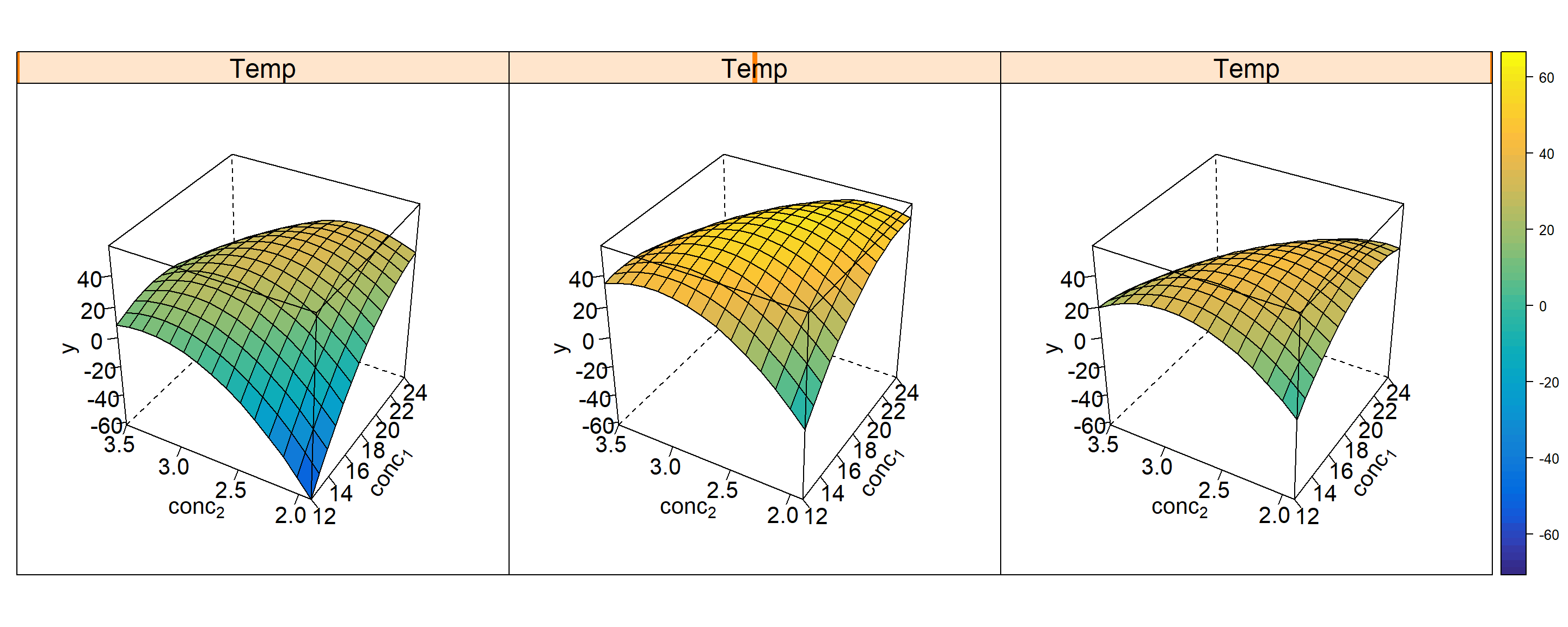
Figure 4.23: Response surface trellis plot \(\hat y=f(conc_{1},conc_{2},Temp)\) of the final CCC design of the polymer data
Response Surface Trellis plot, figure 4.23, and rsm-output clearly reveal a degenerated maximum at conc1=19.4 ; conc2=2.5 ; Temp=146.5, close to the center of the design space. The degree of degeneration (flatness) is indicated by a small first eigenvalue suggesting a flat (degenerated) maximum along the first eigenvector. Almost perpendicular to that direction the maximum drops sharply with the direction indicated by the third eigenvector. Figure 4.24 shows a response surface plot of this maximum with Temp kept at the optimal value and block=0.5, y=f(conc1,conc2)|(temp* = 146.5;block=0.5).
##
## Call:
## rsm(formula = y ~ block + SO(conc1, conc2, Temp), data = x)
##
##                Estimate  Std. Error  t value  Pr(>|t|)
## (Intercept) -2.3552e+03  1.3870e+02 -16.9810 1.296e-05 ***
## block        2.5800e+00  8.6401e-01   2.9861 0.0305856 *
## conc1        5.1108e+01  3.6900e+00  13.8502 3.524e-05 ***
## conc2        4.1220e+02  2.8075e+01  14.6820 2.649e-05 ***
## Temp         1.9095e+01  1.3696e+00  13.9416 3.413e-05 ***
## conc1:conc2 -5.9417e+00  5.0913e-01 -11.6703 8.115e-05 ***
## conc1:Temp  -1.0900e-01  2.0365e-02  -5.3523 0.0030584 **
## conc2:Temp  -6.8250e-01  1.5274e-01  -4.4685 0.0065887 **
## conc1^2     -5.2111e-01  4.8001e-02 -10.8563 0.0001151 ***
## conc2^2     -3.9188e+01  2.7000e+00 -14.5137 2.803e-05 ***
## Temp^2      -5.2100e-02  4.3201e-03 -12.0600 6.920e-05 ***
## ---
## Signif. codes:  0 '***' 0.001 '**' 0.01 '*' 0.05 '.' 0.1 ' ' 1
##
## Multiple R-squared:   0.99,  Adjusted R-squared:   0.97
## F-statistic:  49.5 on 10 and 5 DF,  p-value: 0.0002279
##
## Analysis of Variance Table
##
## Response: y
##                         Df Sum Sq Mean Sq F value    Pr(>F)
## block                    1  26.63  26.626  8.9166 0.0305856
## FO(conc1, conc2, Temp)   3 161.01  53.669 17.9732 0.0041420
## TWI(conc1, conc2, Temp)  3 551.86 183.954 61.6038 0.0002273
## PQ(conc1, conc2, Temp)   3 738.75 246.249 82.4658 0.0001117
## Residuals                5  14.93   2.986
## Lack of fit              4  12.60   3.149  1.3501 0.5620374
## Pure error               1   2.33   2.333
##
## Stationary point of response surface:
##      conc1      conc2       Temp
##  19.381044   2.514217 146.509245
##
## Eigenanalysis:
## eigen() decomposition
## $values
## [1]  -0.04585026  -0.29742296 -39.41743789
##
## $vectors
##                [,1]        [,2]         [,3]
## conc1 -1.137565e-01  0.99058480 -0.076165710
## conc2 -2.767632e-05 -0.07666652 -0.997056791
## Temp   9.935087e-01  0.11341956 -0.008748729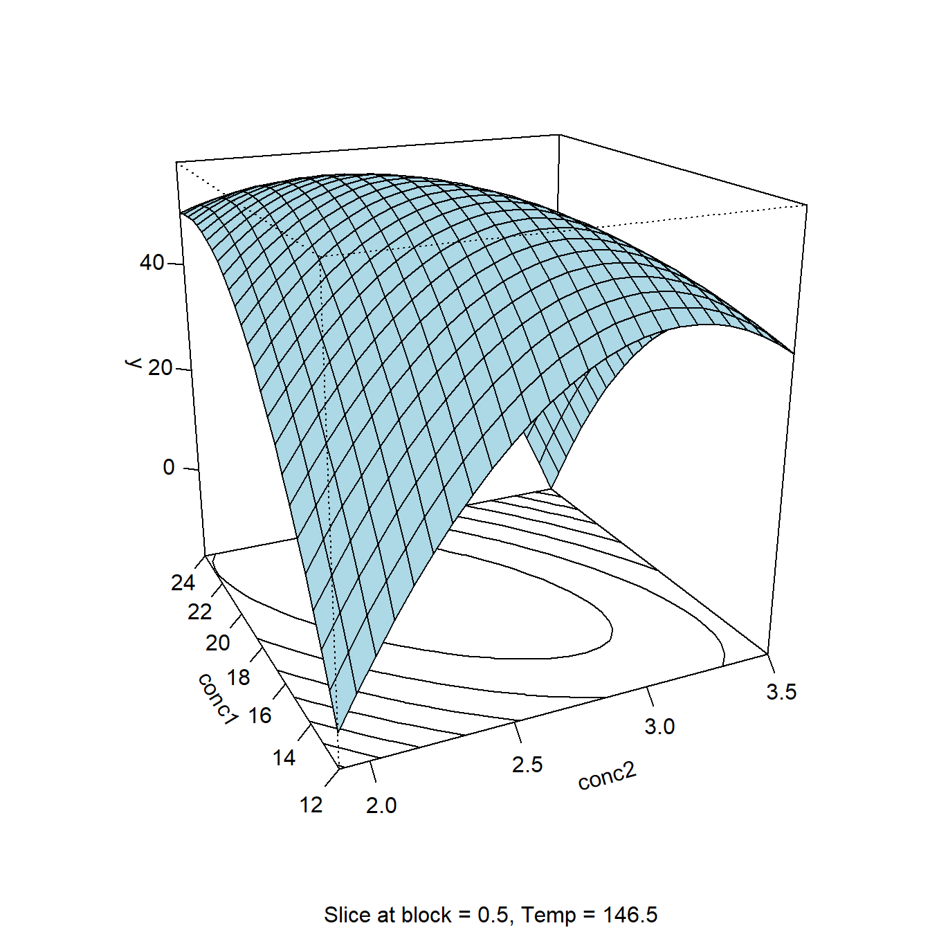
Figure 4.24: Conditional response surface plot \(\hat y = f(conc_{1},conc_{1},Temp)|(Temp=146.5;block=0.5)\) of the CCC polymer data
According to figure 4.24 a decrease in conc1 can be compensated by an increase of conc2 without significantly loosing optimality. However, jointly increasing or decreasing conc1 and conc2 will result in a substantial loss in terms of the objective function y.
Informations about the sensitivity of an optimum in factor space can be very helpful for running a process safe and stable at optimal process conditions.
4.8 Design blocking
Often an experimental design cannot be realized at one stretch and must be divided into temporally disjoint parts. In the sequential use of Central Composite designs for instance, the factorial part is nescessarily realized first and, depending on the outcome, later augmented by star points. Such time gaps can become a source of bias which can, thanks to factorial and star part being orthogonal, controlled by blocking as has been shown in the example, figure 4.16.
Other reasons naturally calling for blocking are experimental heterogeneities introduced by different lab equipment, different staff or different raw material batches.
Many classical designs such as (fractional) factorial and Central Composite designs have the capability of blocking, and more information on how to create blocked factorial and fractional factorial designs, e.g., in R can be found with the function FrF2::blockpick().
Blocking can also be achieved algorithmically with the package AlgDesign and the function optBlock() therein. The following example code demonstrates this functionality by splitting a classical Box-Behnken designs with 16 runs into four blocks of size four. In the simulation with the model \(y = 10B_{2} + 15B_{3} + 20B_{4} + 3x_{1} + 3x_{2} +3x_{3} + 5x_{1}*x_{2} + 5x_{1}^2 - 5x_{2}^2 + 8x_{3}^2 + \epsilon; \ \epsilon \sim N(0,1)\) the OLS estimates agree well with the true model within standard error.
rm(list=ls())
set.seed(1234)
x <- as.data.frame(rsm::bbd(3,randomize=F))[,-c(1,2)]
x <- x[order(runif(nrow(x))),]
rownames(x)  <- NULL
colnames(x) <- paste("x",1:3,sep="")
res <- AlgDesign::optBlock(~ quad(.), x,
      blocksize=rep(4,4), criterion="Dpc", nRepeats=1000)
x       <- res$design
x$Block <- factor(rep(paste("B",1:4,sep=""),each=4))

kappa(model.matrix(~quad(x1,x2,x3), data=x))
## [1] 2.272431kappa(model.matrix(~Block + quad(x1,x2,x3), data=x))## [1] 6.004096x$y <- 10*(x$Block=="B2") + 15*(x$Block=="B3") +
20*(x$Block=="B4") + 3*x$x1 +
3*x$x2 + 3*x$x3 + 5*x$x1*x$x2 +
5*x$x1^2 -5*x$x2^2 +8*x$x3^2 +
rnorm(nrow(x),0,1)
# OLS estimates agree very well with the true parameters
summary(lm(y~Block + (x1+x2+x3)^2 + I(x1^2)+
I(x2^2)+ I(x3^2), data=x))##
## Call:
## lm(formula = y ~ Block + (x1 + x2 + x3)^2 + I(x1^2) + I(x2^2) +
## I(x3^2), data = x)
##
## Residuals:
## 7 10 15 16 2 11 13 14 1 4 8 12
## 0.21677 0.02782 0.24459 -0.48918 -0.02782 -0.09726 -0.06945 0.19453 0.09726 0.43354 -0.31404 -0.21677
## 3 5 6 9
## -0.24459 -0.13890 0.06945 0.31404
##
## Coefficients:
## Estimate Std. Error t value Pr(>|t|)
## (Intercept) -0.65031 0.42418 -1.533 0.222789
## BlockB2 11.15129 0.55539 20.078 0.000270 ***
## BlockB3 16.01074 0.50700 31.580 6.98e-05 ***
## BlockB4 20.55500 0.50700 40.543 3.30e-05 ***
## x1 2.86765 0.24049 11.924 0.001269 **
## x2 3.73879 0.24049 15.547 0.000578 ***
## x3 3.29287 0.19636 16.770 0.000462 ***
## I(x1^2) 4.63003 0.27769 16.673 0.000470 ***
## I(x2^2) -4.74465 0.27769 -17.086 0.000437 ***
## I(x3^2) 8.30608 0.27769 29.911 8.21e-05 ***
## x1:x2 4.70504 0.32065 14.673 0.000687 ***
## x1:x3 -0.12349 0.34010 -0.363 0.740600
## x2:x3 -0.04465 0.34010 -0.131 0.903859
## ---
## Signif. codes: 0 '***' 0.001 '**' 0.01 '*' 0.05 '.' 0.1 ' ' 1
##
## Residual standard error: 0.5554 on 3 degrees of freedom
## Multiple R-squared: 0.9993, Adjusted R-squared: 0.9967
## F-statistic: 375.5 on 12 and 3 DF, p-value: 0.0002009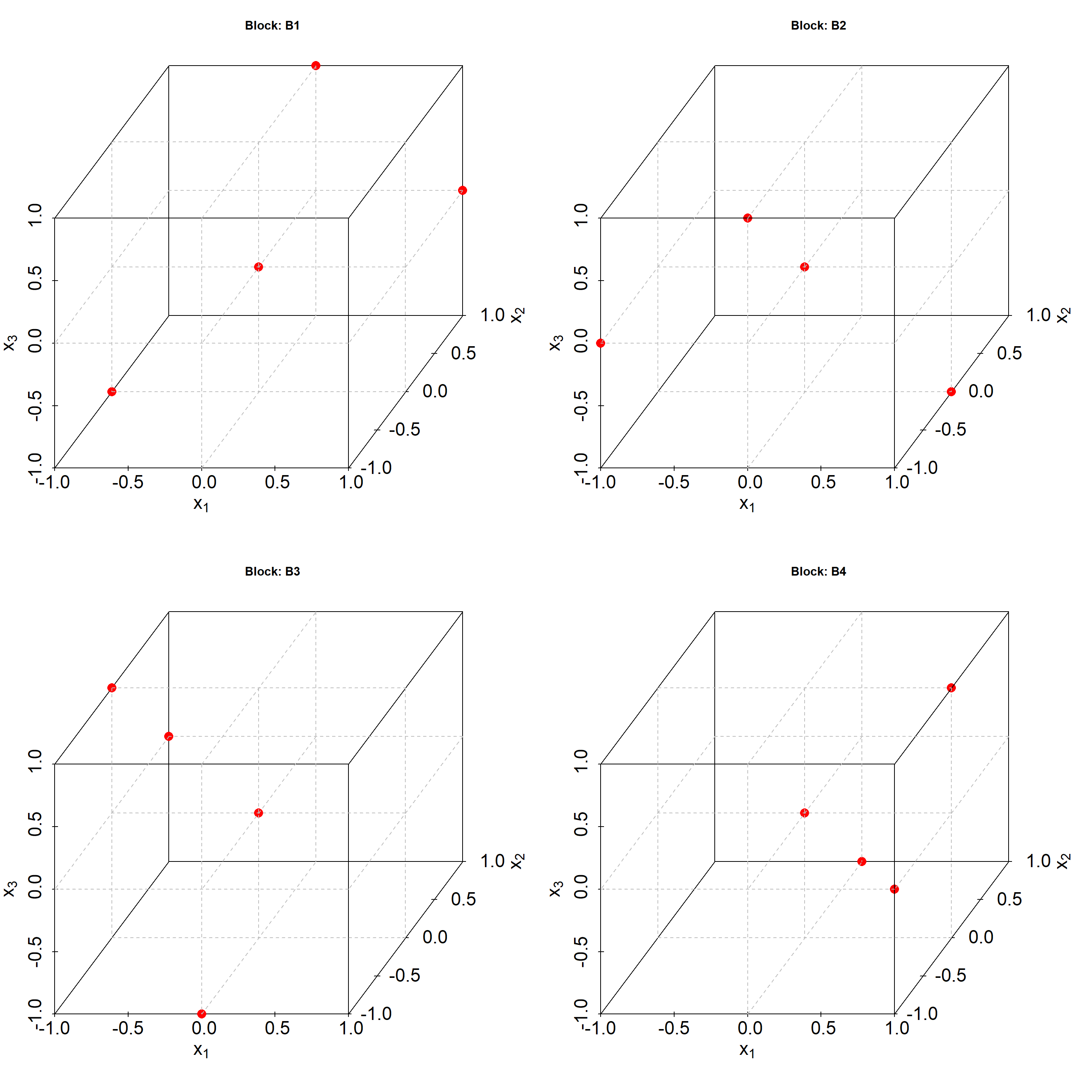
Figure 4.25: Three dimensional Box-Behnken design in four orthogonal blocks
4.9 Variance component analysis
All models and designs discussed to this point aim at estimating the true, however unknown effects \(\beta_{i}\) in a linear parametric model of the general form \(y=\sum_{i}\beta_{i}\cdot g_{i}(x_{1},x_{2},...x_{K}) + \epsilon\) with gi() belonging to a linear, bilinear or quadratic class of transformations. Because the true parameters are estimated from a finite sample, the estimates \(\hat \beta_{i}\) become itself uncertain with good designs minimizing this uncertainty. The parameters \(\beta_{i}\) are also called “fixed effects” and the residuals are the so-called “random effects”, and OLS estimates both, random and fixed effects, with least squares. In this process the residuals, the random effects, are only a by-product, required for judging the reliability of the fixed estimates \(\hat \beta_{i}\). OLS is a member of the so called mixed models. These are models comprising fixed and random effects, although, for historical reasons, OLS is usually subsumed as a linear least squares method. It is not the place here to discuss mixed models, rather the special method of Variance Component Analysis (VCA) will be discussed, as VCA has very wide use in the applied sciences for detecting the sources of variance in process chains.
The elements of VCA can be understood from figure 4.26 which shows a three step process consisting of process, sampling and (analytical) analysis. Each steps is a source of variance contributing to the final variance \(\sigma_{total}^2=\sum_{i=1}^3\sigma_{i}^2\). Now, when a process is running out-of-spec with \(\sigma_{total}^2\) too large38, VCA can be exceedingly helpful in identifying the major sources of variance in the process chain, that is the step presumably causing the problems.
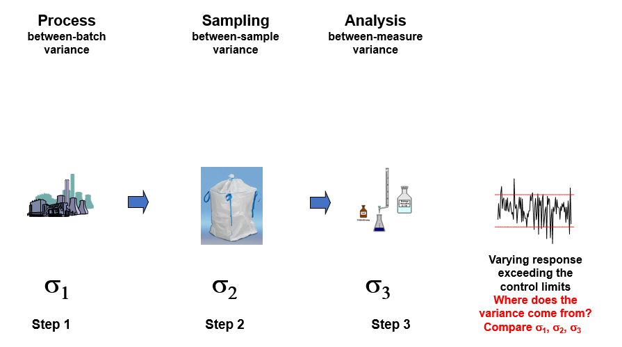
Figure 4.26: Variance components of a three step process with variance component \(\sigma_{1}, \sigma_{2}, \sigma_{3}\)
We shall introduce the key ideas of VCA with a simulated examples, thereby making the data generating process fully transparent.
The random effect model generating the data yijk39 may be written \[y_{ijk}=\beta_{0} + \alpha_{i} + \beta_{ij} + \epsilon_{ijk} \] \[ \alpha_{i} \sim N(0,\sigma_{1}) \] \[ \beta_{ij} \sim N(0,\sigma_{2}) \] \[ \epsilon_{ijk} \sim N(0,\sigma_{3})\] The following R-code generates a sample of (Nbatch=3 x Nsample=3 x Nanalysis~=3)=27 observations with variance components \(\sigma_{batch}=15; \sigma_{sample}=5; \sigma_{analysis}=1\). The result is a nested random effect design with the factor levels of sample nested within batch and analysis nested within sample. The model hierarchy is reflected by the three loops generating the data with the outermost loop, batch, representing the highest and the innermost loop, analysis, representing the lowest hierarchical level. The simulated data set is listed in table 4.14.
Figure 4.27 shows the model hierarchy of a 23 design.
rm(list=ls())
set.seed(123)
sigma1 <- 15
sigma2 <- 5
sigma3 <- 1
x <- NULL
for (batch in (1:3)) {
  alpha <- rnorm(1,0,sigma1)
  for (sample in (1:3)) {
    beta <- rnorm(1,0,sigma2)
    for (analysis in (1:3)) {
      epsilon <- rnorm(1,0,sigma3)
     x <- rbind(x,data.frame(batch,sample,
                analysis,y=alpha+beta+epsilon))
    }
  }
}
x  <- data.frame(obs=1:nrow(x),x)
knitr::kable(
  x, booktabs = TRUE,row.names=F,digits=2,align="c",
caption = 'Nested random effect design on $3^3$ levels')| obs | batch | sample | analysis | y |
|---|---|---|---|---|
| 1 | 1 | 1 | 1 | -8.00 |
| 2 | 1 | 1 | 2 | -9.49 |
| 3 | 1 | 1 | 3 | -9.43 |
| 4 | 1 | 2 | 1 | 0.63 |
| 5 | 1 | 2 | 2 | -1.10 |
| 6 | 1 | 2 | 3 | -0.52 |
| 7 | 1 | 3 | 1 | -9.41 |
| 8 | 1 | 3 | 2 | -10.28 |
| 9 | 1 | 3 | 3 | -10.23 |
| 10 | 2 | 1 | 1 | 0.67 |
| 11 | 2 | 1 | 2 | -0.62 |
| 12 | 2 | 1 | 3 | -3.09 |
| 13 | 2 | 2 | 1 | 4.69 |
| 14 | 2 | 2 | 2 | 4.10 |
| 15 | 2 | 2 | 3 | 4.95 |
| 16 | 2 | 3 | 1 | -4.20 |
| 17 | 2 | 3 | 2 | -4.09 |
| 18 | 2 | 3 | 3 | -5.16 |
| 19 | 3 | 1 | 1 | 12.20 |
| 20 | 3 | 1 | 2 | 14.59 |
| 21 | 3 | 1 | 3 | 13.76 |
| 22 | 3 | 2 | 1 | 11.99 |
| 23 | 3 | 2 | 2 | 11.97 |
| 24 | 3 | 2 | 3 | 11.91 |
| 25 | 3 | 3 | 1 | 16.56 |
| 26 | 3 | 3 | 2 | 15.95 |
| 27 | 3 | 3 | 3 | 15.70 |
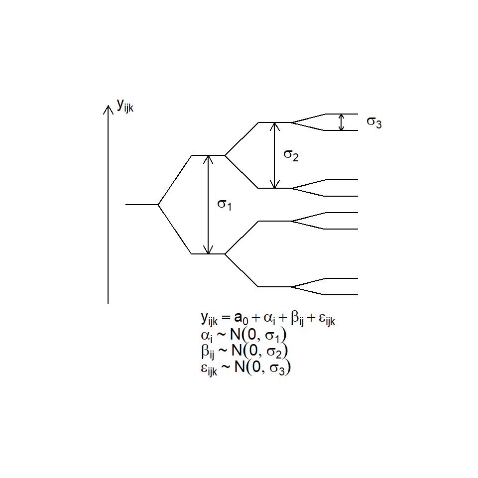
Figure 4.27: Hierarchy of a nested \(2^3\) design with variance components \(\sigma_{1} > \sigma_{2} > \sigma_{3}\).
The simulated example from above becomes in reality a design problem consisting of three random sampling steps, namely
- From the batch process select three batches at random and record the batch ID, i=1,2,3.
- From each batch i=1,2,3 take three samples j=1,2,3 at random and record the ID i,j.
- Analyse each of the nine samples from above three times k=1,2,3 and record the obtained values yijk.
The experimental data thus obtained will be similar to table 4.14, and the objective is now to estimate the variance components \(\sigma_{1}\),\(\sigma_{2}\) and \(\sigma_{3}\) from the data. In R there are many packages and functions for doing variance component analysis. Skipping any theory here40, the package lme4 and VCA will be used with the two functions lme4::lmer() and VCA::anovaVCA(). In both functions the nested effect structure is specified by ~batch/sample (read “sample nested within batch”), and the last factor (analyse) is omitted for being identical with the residual of the model, \(\epsilon_{ijk}\). The generic R-function confint() gives 95% confidence intervalls of the variance components.
library(lme4)
summary(res  <- lmer(y~ 1 +  (1|batch/sample), data=x ))
## Linear mixed model fit by REML ['lmerMod']
## Formula: y ~ 1 + (1 | batch/sample)
## Data: x
##
## REML criterion at convergence: 111.6
##
## Scaled residuals:
## Min 1Q Median 3Q Max
## -2.2756 -0.4212 -0.0073 0.4479 1.8189
##
## Random effects:
## Groups Name Variance Std.Dev.
## sample:batch (Intercept) 17.5050 4.1839
## batch (Intercept) 102.1885 10.1088
## Residual 0.8404 0.9167
## Number of obs: 27, groups: sample:batch, 9; batch, 3
##
## Fixed effects:
## Estimate Std. Error t value
## (Intercept) 2.373 6.003 0.395confint(res)## 2.5 % 97.5 %
## .sig01 2.5641739 8.440086
## .sig02 3.4991394 24.955135
## .sigma 0.6827736 1.322468
## (Intercept) -11.3129630 16.058027VCA::anovaVCA(y~batch/sample,x)##
##
## Result Variance Component Analysis:
## -----------------------------------
##
## Name DF SS MS VC %Total SD CV[%]
## 1 total 2.475824 120.537577 100 10.978961 462.751894
## 2 batch 2 1946.169529 973.084764 102.192132 84.78031 10.109012 426.08447
## 3 batch:sample 6 320.133475 53.355579 17.505067 14.522498 4.183906 176.347321
## 4 error 18 15.126806 0.840378 0.840378 0.697192 0.916721 38.638863
##
## Mean: 2.372537 (N = 27)
##
## Experimental Design: balanced | Method: ANOVAThe variance components are estimated to be \(\sigma_{batch}=10.1(15)\), \(\sigma_{sample}=4.2(5)\) and \(\sigma_{analyse}=0.9(1)\) with true values given in parenthesis. The confidence intervals are very wide, namely \(0 \leq \sigma_{sample} \leq \infty\), \(3.5 \leq \sigma_{batch} \leq 25\) and \(0.7 \leq \sigma_{analyse} \leq 1.3\). The large uncertainty is a result of the small sample size. Nevertheless, the estimates are of the right order of magnitude. Based on these simulated results, the conclusion is to scrutinize the process step (labelled “batch”) more closely, as this step is responsible for 85% of the variance of yijk.
Reference
George E.P. Box, Norman R. Draper. 1987. Empirical Model-Building and Response Surfaces. 1st ed. John Wiley & Sons.
It should be noted that from a practical point of view the different optimization criteria are all similar and will give “good” designs. From a theoretical point of view they differ by giving different weight to certain statistical properties of the design, such as minimizing the average error of the estimates (A) or minimizing the maximum prediction error of the model (G-optimality). A good compromise over these properties is given by the D-criterion which seeks to minimize the determinant of \((\boldsymbol {X^{T}X)^{-1}}\). Geometrically, this is equivalent to minimizing the confidence (hyper-)ellipsoid of the parameter estimates.↩
A scientific experiment can be conceived as a question asked to nature. The answer and the precision of her answer is not independent from the question being asked. DoE, to borrow from this simile, amounts to asking most precise questions.↩
When one column in the design matrix, say xi, can be approximately expressed as a linear function of other columns xj, \(x_{i}=\sum_{j,j \ne i}a_{j} \cdot x_{j} + \epsilon\).↩
ANalysis Of VAriance↩
ANalysis of COVAriance↩
There are six cat-co.cat combinations (cat and co.cat are on three and two levels, respectively) leading to a total of 6x5/2 contrasts.↩
Note that in R the formula expression (…)^k will expand all factors in the argument list into main effects plus k-way interactions.↩
\[activity = 5 \cdot I(cat=A) - 1 \cdot I(cat=B) - 2 \cdot I(cat=C) \] \[ - 1 \cdot I(cat=A) \cdot co.cat + 2 \cdot I(cat=B) \cdot co.cat + 3 \cdot I(cat=C) \cdot co.cat + \epsilon; \] \[ \epsilon \sim N(0,1)\]↩
Stratified analysis means: Take the data of each cat individually and do OLS with each data stratum A,B,C separately.↩
Note that a square term in R formula notation must be specified as “I(x1^2)” with the “as.is” function I(); see “?lm” and the R-introduction for more details on how to specify formula objects in R↩
Note that the estimates of the square terms, I(x1^2), I(x4^2), are the same, despite x1 and x2 being different.↩
In R formula language the interaction term between \(x_{1}\) and \(x_{2}\) is written \(x_{1} \colon x_{2}\), rather than \(x_{1} \cdot x_{2}\).↩
A model matrix of dimension 11x21 allows estimation of 11 linear independent parameters. The remaining 10 parameters are linear functions of these independent parameters. Hence, 10 out of 21 eigenvalues will be zero.↩
Hierarchical model building is the process of including higher order model terms, such as square and interaction terms, not before their corresponding main effects have been included.↩
“The objective of this investigation was to explore reaction conditions yielding close to maximal elasticity for a certain polymer. At this stage of the enquiry, the variables of importance had been narrowed down to three. ….” (George E.P. Box, Norman R. Draper 1987) pp. 306-309↩
Often and unjustified, the staff of the last stage is taken responsible for the process variability. Here, VCA can help to settle the debate by quantifying the individual variance components of the different process steps↩
The indices i,j,k refer to batch (process), sample and analysis in figure 4.26, so, e.g., y213 denotes the third analysis of the first sample from the second batch.↩
The basic idea for solving parametric models in statistics is finding the parameters under which the data in hand is the most likely realization. With D denoting the data and \(a_{i}\) the model parameters, the optimization problem is \(\max_{a_{i}} Prob(D|a_{i})\), a method called Maximum Likelihood (ML). It can be shown that OLS belongs to this class.↩