2 Basics of empirical model building
Statistics is the mathematical science dealing with uncertainty and change. There are many fields of modern statistics, but the branch of empirical model building became particular popular with the advent of modern machine learning methods. Machine learning and empirical model buiding aims at deriving functional representations (mathematical models) of large multidimensional data sets which can then be used for deriving insight into the data and/or predicting new cases. The following two chapters will introduce into the basic concepts of empirical model building, the underlying assumptions and some problems associated with this field of application.
2.1 Model building with historical data
It is an everyday experience that everything in the world is in a state of constant flux and subject to permanent change, a state schematically depicted in figure 2.1
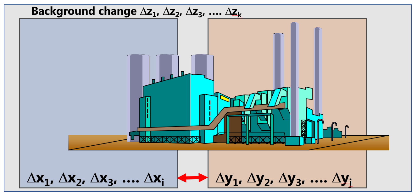
Figure 2.1: Analysing change in front of a changing background
The changing entities (variables) in 2.1 can be conceptually divided into X-, Y- and Z-variables:
\[\Delta X: \{\Delta x_{1}, \Delta x_{2}... \Delta x_{I}\}; \] \[ \Delta Y: \{\Delta y_{1}, \Delta y_{2}... \Delta y_{J}\}; \] \[\Delta Z: \{\Delta z_{1}, \Delta z_{2}... \Delta z_{K}\}; \] \[ I,J,K \in \mathbb N \] \[ X,Y,Z \in \mathbb R\]
In this notation the X-variables are considered to be the “independent” variables influencing the Y-variables (the responses \(\Delta Y\) responding to the changing X-variables, \(\Delta X\)), while background variables \(\Delta Z\) are assumed unkown and changing, too. Defining X,Y,Z for historical data is usually done based on scientific ground and knowledge of the system, because no statistical analysis of observational data can make such an assignment. In this model all variables are assumed changing, indicated by the prefix operator \(\Delta\).
Without loss of generality the relationship of one particular response \(\Delta y\) with \(\Delta X\), \(\Delta Z\) and the link function \(F()\) can be written:
\[\begin{equation} \Delta y = F(\Delta X,\Delta Z) = F(\Delta x_{1}, \Delta x_{2}... \Delta x_{I};\Delta z_{1}, \Delta z_{2}... \Delta z_{K} ) \tag{2.1} \end{equation}\]Under the assumption that background variables \(\Delta Z\) do not affect foreground variables \(\Delta X\), equation (2.1) can be factorized into \(f()\) and \(g()\)1
\[\begin{equation} \Delta y = f(\Delta X) + g(\Delta Z) = f(\Delta x_{1}, \Delta x_{2}... \Delta x_{I}) + g(\Delta z_{1}, \Delta z_{2}... \Delta z_{K} ) \tag{2.2} \end{equation}\] Under the weak assumption that the background change \(\Delta Z\) is sufficiently small and with \(a_{k}\) being the first order derivative of \(g()\) at \(z_{k}\), the second term in (2.2) can be simplified\[\begin{equation} \Delta y = f(\Delta X) + \sum_{k=1}^{K} a_{k}\cdot\Delta z_{k} = f(\Delta x_{1}, \Delta x_{2}... \Delta x_{I}) + \sum_{k=1}^{K} a_{k}\cdot\Delta z_{k} \tag{2.3} \end{equation}\] By the Central Limit Theorem - sums of arbitrarily distributed random variables are asymptotically normal distributed, \(\sum_{k=1}^{K} a_{k}\cdot\Delta z_{k} = \epsilon \sim N(0,\sigma^2)\)2 - (2.3) can be further simplified and becomes \[\begin{equation} \Delta y = f(\Delta X) + \epsilon = f(\Delta x_{1}, \Delta x_{2}... \Delta x_{I}) + \epsilon; \ \epsilon \sim N(0,\sigma^2) \tag{2.4} \end{equation}\]
(2.4) is the formula usually found in text books on statistical learning and empirical model building: The observed response \(\Delta y\) is a function of the influential factors \(\Delta X\) plus some random noise from a normal distribution with unknown variance \(\sigma^2\). In deriving the base equation of empirical model building, \(\Delta y=f(\Delta X)+\epsilon\), two strong assumptions were made, namely
- Factorization of (2.1)
- This is a very strong assumption and ensures that the model f() is invariant with respect to the backgound (space and time). It ensures generalisability of f() in space and time, an assumption usually taken for granted of the laws of nature.
- The assumption of normality in (2.4)
- Depending on the dimension K of Z and K being sufficiently large, and the variability of the background variables Z, the normality hypothesis might often be an assumption too tight. However, non-normal data can be handled within the framework of empirical model building, hence normality of the random term is not a crucial hypothesis.
However, these limitations are by far not the most crucial when working with historical data.
What can turn historical model building and inference3 into a nightmare are the mutual dependencies between the X-variables which will render the model building process often difficult and inconclusive. From a more fundamental point of view, working with historical data suffers from not knowing the source of variance \(\Delta X\): There is change \(\Delta X\) and \(\Delta Y\) in front of a changing background \(\Delta Z\), and it remains unclear from what source the change in \(\Delta X\) has arisen4 (and the same is, of course, true for \(\Delta Z\) and \(\Delta Y\)). Compared with this problem, the problem of finding an adequate functional representation \(f()\) between \(\Delta y\) and \(\Delta X\) is a minor one that can be solved with modern machine learning methods5.
2.2 Model building based on well-designed data
In the previous chapter 2.1, the basic elements of empirical model building were introduced. All concepts derived there also apply to DoE with one fundamental difference: The source of variance \(\Delta X\) in a well-controlled experiment is known with the experimenter becoming the indubitable source of that variance. This process is schematically depicted in figure 2.2.
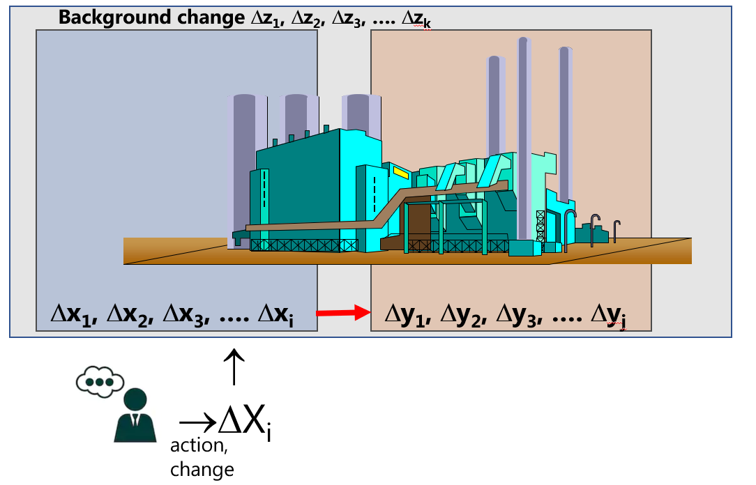
Figure 2.2: Introduction of variance by an agent with DoE
The researcher selects from a set of potential variables X a subset, X’, deemed relevant for the problem at hand and varies these parameters (that is \(X' \rightarrow \Delta X'\)) within carefully chosen boundaries \(\Delta\) with an experimental design while trying to keep the background variables, if known, as constant as possible
(\(Z=const. \rightarrow \Delta Z=0\)).
The X-variables are deliberately and systematically varied to study, how this variation affects Y6. By carefully selecting the support point in a linear space \(\mathbb{R}^N\) the effects \(\Delta X\) can be separated from the background noise and quantified as an analytical expression \(\Delta y = f(\Delta X) + \epsilon\)
The science of designing and analysing multivariate experiments in N-dimensional space \(\mathbb{R}^N\) with the R-software will be elucidated in the following chapters.
In essence, the process just described is the scientific method usually attributed to Bacon (1561-1626) who allegedly expressed this thought first. It boils down to the simple recipe: Bring together new conditions in a controlled experiment and see what condition(s) arise(s) from that action.
Factorization requires that all mixed partial derivaties must vanish, formally \[\frac{\partial^k}{\partial z_{1}... \partial z_{k}} \biggl( \frac{\partial^i f(x_{1},...x_{I}; z_{1},... z_{K}}{\partial x_{1}... \partial x_{i}} \biggr) = 0; \forall \ i,k \leq I,K \] , so background variables Z are not allowed to moderate foreground variables X thereby rendering the model time-invariant.↩
Inference refers here to the process of separating significant from nonsignificant variables. The latter are usually excluded from model building as non-informative↩
An example might be helpful at this point. Say we have some chemical process data consisting of selectivity and temperature. From first principles we know that temperature affects selectivity and it seems natural to set up the model selectivity=f(temperature) with selectivity being the response Y and temperature being the independent factor X. Here, the assumption is that the variability of the response results from the variability of X. However, if there is a controller in the plant controlling the temperature as a function of the selectivity our model assumption is wrong, because the variability of temperature results from the variability of the selectivity and not vice-versa. This is not something the data can tell. This information must come from outside, from the context of the data. In addition, the process might be affected by ambient conditions unknown to the plant operators, some “lurking” background variables Z.↩
In chapter 7 the Random Forest as a flexible machine learning method will be used for analysing historical data.↩
The concept of causality is based on the somewhat hidden assumption that change always results from and leads to change. In statistical terms: Without variation no co-variation. Knowledge of whether and how entities are related is based on change.↩