Chapter 3 Modeling
In this chapter, we will use two different metrics to build and assess our models:
- Accuracy
- Receiver Operating Characteristic (ROC)
3.1 Data splitting and data balancing
We have seen in the EDA that variables age, amount and duration are right skewed. Therevore, we proceed to a log transformation of those features. In order to normalize them, we scale those variables.
Then, we split the dataset into a training test and a test set. The training set is used to find optimal hyperparameters when tuning them. For this process, we will use a 5-fold cross-validation applied on the training set. The test set will be used to compare and evaluate the models in order to know how well the models can generalize new data.
Therefore, we split the database into two parts:
- Training set (80%)
- Test set (20%)
#First we tried to scale the data to normalize them
german <- german %>% mutate(LogAge = log(age),
                    Log1pAmount = log1p(amount),
                    Log1pDuration = log1p(duration))

german$LogAgestd <- scale(german$LogAge)
german$Log1pAmountstd <- scale(german$Log1pAmount)
german$Log1pDurationstd <- scale(german$Log1pDuration)


german <- german %>% select(-age, -amount, -obs, -duration, -LogAge, -Log1pAmount, -Log1pDuration)


#Splitting the dataset into a training (80%) and a test set (20%)
set.seed(245156)
index <- sample(x=1:2, size = nrow(german), replace = TRUE, prob = c(0.8, 0.2))
german.tr <- german[index == 1,]
german.te <- german[index == 2,]
In the EDA, we observed an unbalanced dataset. We have much more credits classified as good (700) than bad (300). In order to have a correct prediction, we need to balance the number of good et bad credits in our training set. It will thus balance the sensitivity and the specificity. Because the importance is to predict well risky credits in order to avoid huge losses whithin the company, we need a good specificity but the balance between both measures is important.
As we can see with the risk variable in the training set, data are unbalanced.
#As we can see with the risk variable, the data are unbalanced
table(german.tr$risk) %>% kable(align = "c", col.names = c("Variable", "Frequence"))| Variable | Frequence |
|---|---|
| bad | 236 |
| good | 569 |
Below, we display the number of bad and good credits after having balanced the training set.
#Balancing the data
n.bad <- sum(german.tr$risk == "bad")
n.good <- sum(german.tr$risk == "good")

set.seed(245156)
index.bad <- which(german.tr$risk == "bad")
index.good <- sample(x = which(german.tr$risk == "good"), size = n.bad, replace = FALSE)

german.tr.bal <- german.tr[c(index.bad, index.good),]

table(german.tr.bal$risk) %>% kable(align = "c", col.names = c("Variable", "Frequence"))| Variable | Frequence |
|---|---|
| bad | 236 |
| good | 236 |
3.2 Accuracy metric: training and fitting the models
By using the CARET package, we need some parameters first to train our models. It will be used for each model with accuracy metric.
As mentioned before, we will use a five cross-validation to subset the training set (into a validation set) in order to assess how well the model will generalize new data on the test set.
train_control <- trainControl(method = "cv", number = 5)
metric <- "Accuracy"
3.2.1 Logistic regression
A logistic regression is a binary classifier and is used for output with two classes.
We will use the AIC selection in order to have a model with more significant variables.
set.seed(123)

fit_glm_AIC = train(
  form = risk ~ .,
  data = german.tr.bal,
  trControl = train_control,
  method = "glmStepAIC",
  metric = metric,
  family = "binomial"
)
Our confusion matrix plot shows that sensitivity and specificity are quite well balanced. However, accuracy is quite low.
pred_glm_aic <- predict(fit_glm_AIC, newdata = german.te)
cm_glm_aic <- confusionMatrix(data = pred_glm_aic, reference = german.te$risk)
draw_confusion_matrix(cm_glm_aic)
By analysing more precisely our model, we observe that it contains insignificant variables according to the p-values. We decided to remove them from the model.
pvalues<- fit_glm_AIC$finalModel
pvalues %>% tidy() %>%
  select(-statistic) %>%
  mutate(p.value = paste(round(p.value, 4), pval_star(p.value))) %>%
  kable(digits = 3,
    col.names = c("Parameter", "Estimate", "Standard Error", "P.value")
  ) %>%
kable_styling(bootstrap_options = "striped")| Parameter | Estimate | Standard Error | P.value |
|---|---|---|---|
| (Intercept) | -1.547 | 0.547 | 0.0047 ** |
| chk_acct | 0.516 | 0.095 | 0 *** |
| history | 0.449 | 0.122 | 2e-04 *** |
| used_car | 1.571 | 0.432 | 3e-04 *** |
| radio.tv | 0.431 | 0.270 | 0.1101 |
| education | -1.215 | 0.581 | 0.0363 * |
| sav_acct | 0.199 | 0.079 | 0.0119 * |
| employment | 0.202 | 0.098 | 0.0395 * |
| male_single | 0.537 | 0.241 | 0.0256 * |
| guarantor | 0.955 | 0.491 | 0.0519 |
| prop_unkn_none | -0.657 | 0.328 | 0.045 * |
| other_install | -0.508 | 0.284 | 0.0733 |
| rent | -0.651 | 0.301 | 0.0303 * |
| num_credits | -0.342 | 0.219 | 0.1182 |
| job | -0.449 | 0.193 | 0.02 * |
| telephone | 0.487 | 0.258 | 0.0593 |
| foreign | 1.405 | 0.705 | 0.0462 * |
| Log1pDurationstd | -0.538 | 0.122 | 0 *** |
The logistic regression has no parameter to tune unlike other models that we will use.
#Logistic regression
set.seed(123)

fit_glm_AIC = train(
  form = risk ~ chk_acct + history + used_car + education + sav_acct + employment + male_single +
  prop_unkn_none + rent + job + foreign + Log1pDurationstd,
  data = german.tr.bal,
  trControl = train_control,
  method = "glmStepAIC",
  metric = metric,
  family = "binomial"
)
pred_glm_aic <- predict(fit_glm_AIC, newdata = german.te)
cm_glm_aic <- confusionMatrix(data = pred_glm_aic, reference = german.te$risk)
draw_confusion_matrix(cm_glm_aic)
Even if our final model decreased in accuracy, the gab between sensitivity and specificity is smaller. Moreover, because we removed insignificant variables, the final model makes more sense.
Finally, we compute the VIF coefficients to look for multicollineratity which is not the case as we can see below (VIF coefficients <5).
vif(pvalues) %>% kable(col.names = "VIF Coefficient") %>% kable_styling(bootstrap_options = "striped")| VIF Coefficient | |
|---|---|
| chk_acct | 1.101125 |
| history | 1.267096 |
| used_car | 1.200954 |
| radio.tv | 1.124241 |
| education | 1.085464 |
| sav_acct | 1.057604 |
| employment | 1.142739 |
| male_single | 1.169750 |
| guarantor | 1.126230 |
| prop_unkn_none | 1.189223 |
| other_install | 1.078695 |
| rent | 1.094990 |
| num_credits | 1.317337 |
| job | 1.372632 |
| telephone | 1.308709 |
| foreign | 1.061026 |
| Log1pDurationstd | 1.155109 |
3.2.2 Nearest neighbour classification (KNN)
The K-NN model computes the distance between observations in order to classify them. It means that the model counts the classes of the K nearest instances and the class with the most observations is selected for the K observations.
#KNN
set.seed(456)
fit_knn_tuned = train(
  risk ~ .,
  data = german.tr.bal,
  method = "knn",
  metric = metric,
  trControl = train_control,
  tuneGrid = expand.grid(k = seq(1, 101, by = 1))
)
We are looking for the optimal K.
plot(fit_knn_tuned)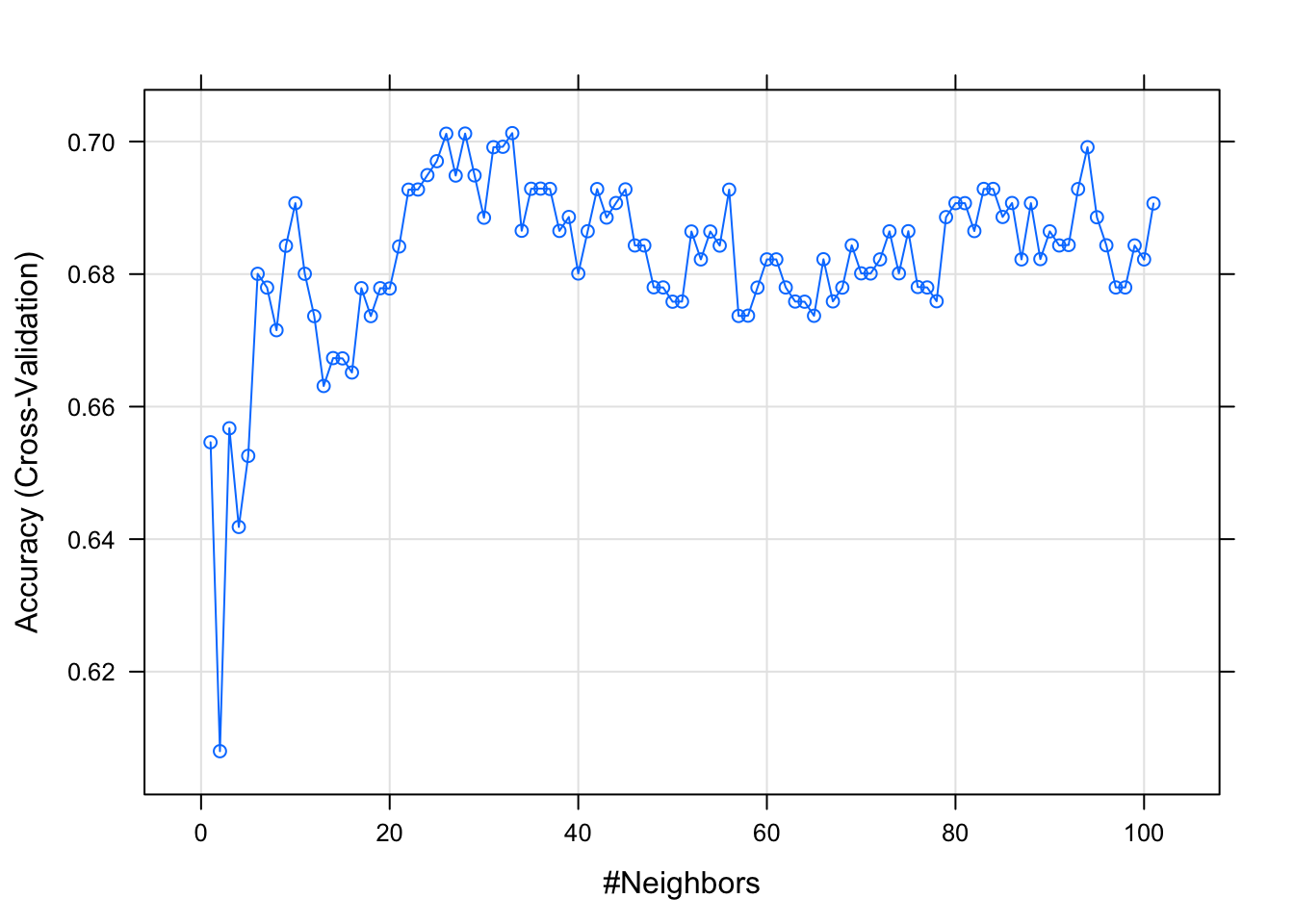
K <- fit_knn_tuned$finalModel$k
paste("The optimal K of our model is", K) %>% kable(col.names = NULL, align = "l")| The optimal K of our model is 33 |
pred_knn <- predict(fit_knn_tuned, newdata = german.te)
cmknn <- confusionMatrix(data = pred_knn, reference = german.te$risk)
draw_confusion_matrix(cmknn)
The KNN model makes better predictions than the logistic regression. In addition, the scores for sensitivity and specificity are very well balanced.
3.2.3 Support Vector Machine (SVM)
The model, considered as a separation method, consists in looking for the linear optimal separation of the hyperplane in order to classify the observations.
With the CARET package, we can only tune the cost hyperparameter. The cost controls the tolerance to bad classification and corresponds to the smoothing of the border that classifies the observations. The larger is the cost (border is not smooth), the fewer missclassifications are allowed. If the cost is too large, it can lead to overfitting.
#SVM
hp_svm <- expand.grid(cost = 10 ^ ((-2):1))
set.seed(1953)
fit_svm <- train(
  form = risk ~ .,
  data = german.tr.bal,
  trControl = train_control,
  tuneGrid = hp_svm,
  method = "svmLinear2",
  metric = metric
)
C <- fit_svm$finalModel$cost
paste("The optimal cost for our model is", C) %>% kable(col.names = NULL, align="l")| The optimal cost for our model is 0.01 |
pred_svm <- predict(fit_svm, newdata = german.te)
cmsvm <- confusionMatrix(data = pred_svm, reference = german.te$risk)
draw_confusion_matrix(cmsvm)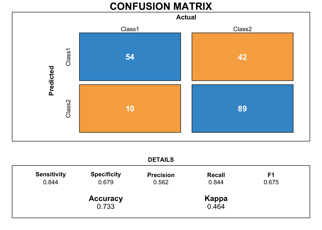
The score for sensitivity is much higher than for specificity. Sensitivity measures the proportion of true positives that are correctly identified. Thus, the model predicts more accurately credits that are considered good but has difficulty to predict bad credits. Therefore, this model does not really correspond to our expectations.
3.2.4 Neural network
A neural network combines several predictions of small nodes and contains lots of coefficients (weights) and parameters to tune. Neural networks are over-parametrized by nature and therefore, the solution is quite unstable. In order to avoid overfitting, we will use a weight decay to penalise the largest weights. We will also tune the size of the neural network to find the opimal one.
#Neural network
hp_nn <- expand.grid(size = 2:10,
                     decay = seq(0, 0.5, 0.05))
set.seed(2006)
fit_nn <- train(
  form = risk ~ .,
  data = german.tr.bal,
  trControl = train_control,
  tuneGrid = hp_nn,
  method = "nnet",
  metric = metric,
  verbose=F
)
Below, we display our neural network.
plotnet(fit_nn$finalModel)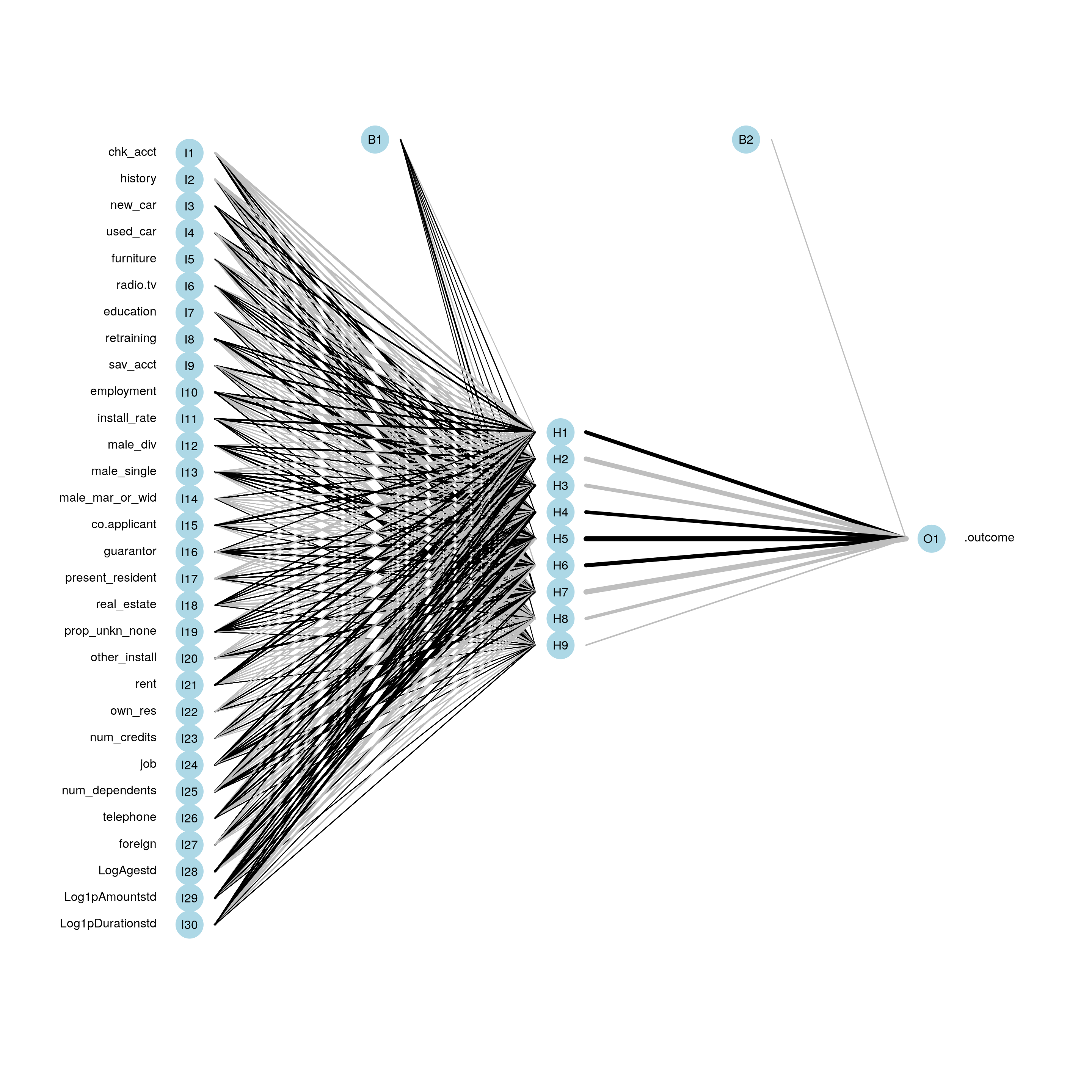
decay <- fit_nn$finalModel$decay
paste("The best neural network has a decay of", decay) %>% kable(col.names = NULL, align="l")| The best neural network has a decay of 0.45 |
arch<- fit_nn$finalModel$n
cat("The model architecture is the following:","\n", "- Number of layers =", length(arch), "\n",
      "- Nodes in the first layer =", arch[1], "\n",
      "- Nodes in the second layer =", arch[2], "\n",
      "- Nodes in the third layer (output) =", arch[3])
## The model architecture is the following:
## - Number of layers = 3
## - Nodes in the first layer = 30
## - Nodes in the second layer = 9
## - Nodes in the third layer (output) = 1pred_nn <- predict(fit_nn, newdata = german.te)
cmnn <- confusionMatrix(data = pred_nn, reference = german.te$risk)
draw_confusion_matrix(cmnn)
Scores of the neural network model do not outperform the scores of the K-NN model.
3.2.5 Linear discriminant analysis (LDA)
The aim of the linear discriminant analysis is to explain and predict the class of an observation according to a linear combination of features that characterizes the classes.
There is no tuning parameter for this model.
#LDA
set.seed(1839)
fit_LDA <- train(risk ~ .,
                 data = german.tr.bal,
                 method = "lda",
                 metric = metric,
                 trControl = train_control)
pred_lda <- predict(fit_LDA, newdata = german.te)
cmlda <- confusionMatrix(data = pred_lda, reference = german.te$risk)
draw_confusion_matrix(cmlda)
Like the SVM model, there is a huge gab between sensitivity and specificity. So this model does not meet our needs as it is only good at predicting good credits.
3.2.6 Random Forest
A random forest model is composed by a multitude of decision trees forming a whole. Each individual tree predicts a class and the class receiving the most votes becomes the prediction model. Thus, the predictions of the individual trees are averaged to get a final prediction. The trees are uncorrelated and operate as a set. Therefore they outperform the individual models. The non-correlation between trees brings some stability to the final prediction.
To tune the model, we will play around the number of trees composing the random forest.
#Random forest
hp_rf <- expand.grid(.mtry = (1:15))
set.seed(531)
fit_rf <- train(
  risk ~ .,
  data = german.tr.bal,
  method = 'rf',
  metric = metric,
  trControl = train_control,
  tuneGrid = hp_rf
)
Here, we display the importance of the variables. We note that the most important variables are not necessarily the same as those chosen in the logistic regression with AIC and p-values.
varImp(fit_rf) %>% plot()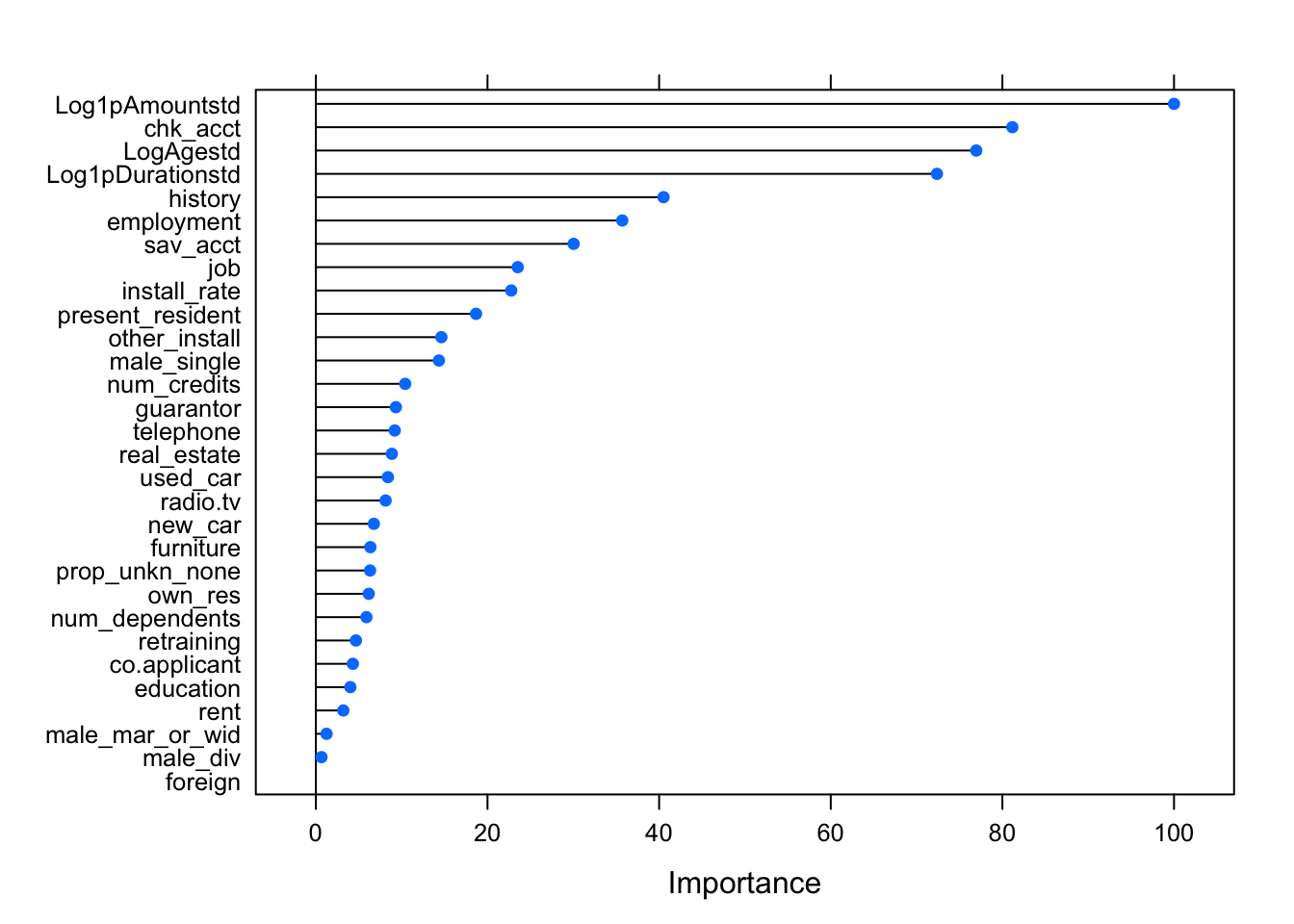
ntree <- fit_rf$finalModel$mtry
paste("Our random forest model is composed by", ntree, "trees") %>% kable(col.names = NULL, align="l")| Our random forest model is composed by 12 trees |
pred_rf <- predict(fit_rf, newdata = german.te)
cmrf <- confusionMatrix(data = pred_rf, reference = german.te$risk)
draw_confusion_matrix(cmrf)
Although the accuracy is close to the score obtained with the KNN model, the difference between specificity and sensitivity is too disparate.
3.2.7 Decision tree
A tree is a graphical representation of a set of rules. The importance of characteristics is clear and relationships can be interpreted.
For the decision tree model, we decided to tune the complexity parameter “cp” to be in the range 0.03 and 0.
The complexity parameter controls the optimal size of the tree. If the cost of adding another variable to the tree from the current node is above the value of the complexity parameter, we stop growing the tree. Therefore, the complexity parameter is the minimum improvement needed in the model at each node.
Because we use the CARET package, we do not need to prune the tree as the tree is already simplified.
#Decision tree
hp_ct <- expand.grid(cp = seq(from = 0.03, to = 0, by = -0.003))

set.seed(1851) #allow repoducibility of the results

fit_ct <- train(
  form = risk ~ .,
  data = german.tr.bal,
  trControl = train_control,
  tuneGrid = hp_ct,
  method = "rpart",
  metric = metric
)
Below, we diplay our final tree. The most important variable is the first used to build the tree. For our tree, the most important variable is “chk_acct” which corresponds to the checking account status.
fancyRpartPlot(fit_ct$finalModel, main = "Regression tree", caption = NULL)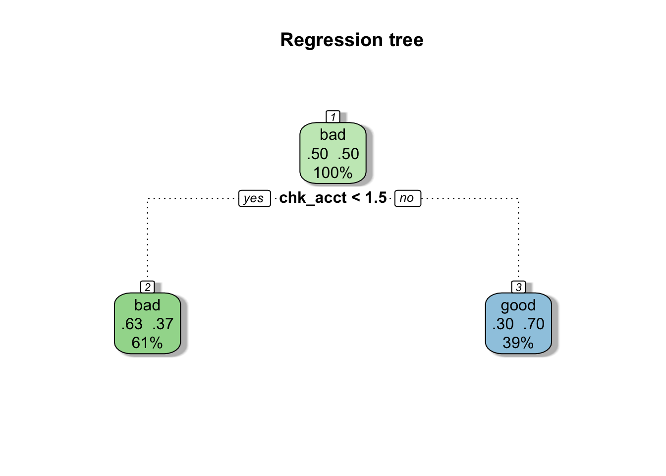
pred_ct <- predict(fit_ct, newdata = german.te)
cmct <- confusionMatrix(data = pred_ct, reference = german.te$risk)
draw_confusion_matrix(cmct)
The confusion matrix demonstrates that the classification tree gets the worst scores so far. The gap between the specificity and the sensitivity is considerable.
3.2.8 Naive Bayes
Naive Bayes model uses a probabilistic approach and allows an interpretation of the features.
The aim is to predict the class of an instance by choosing the class that maximizes the conditional probability given the features.
In order to find the optimal model, we will try to use or not use the kernel density and we will set the laplace smoother value to zero. In addition, the adjust parameter will allow us to adjust the bandwidth of the kernel density. The larger is the number, the more flexible is the density estimate.
#Naive Bayes
hp_nb <- expand.grid(
  usekernel = c(TRUE, FALSE),
  laplace = 0,
  adjust = seq(from = 0.1, to = 5, by = 0.5)
)

set.seed(2013)
fit_nb <- train(
  form = risk ~ .,
  data = german.tr.bal,
  trControl = train_control,
  tuneGrid = hp_nb,
  method = "naive_bayes",
  metric = metric
)
Our best model uses kernel density as we can see on the following graph.
plot(fit_nb)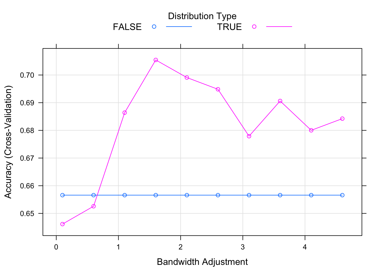
pred_nb <- predict(fit_nb, newdata = german.te)
cmnb <- confusionMatrix(data = pred_nb, reference = german.te$risk)
draw_confusion_matrix(cmnb)
Unlike other previous models, the naive bayes model is better at predicting the bad credits rather than the good ones. Detecting bad risk credits is a important goal of bank employees. Therefore, this model can be useful for them despite the quite low accuracy.
3.2.9 Evaluation of the models
A summary of the scores of each model can be found in the following table.
accuracy<- c(

confusionMatrix(predict.train(fit_glm_AIC, newdata = german.te),
german.te$risk)$overall[1],
confusionMatrix(predict.train(fit_nb, newdata = german.te),
german.te$risk)$overall[1],
confusionMatrix(predict.train(fit_nn, newdata = german.te),
german.te$risk)$overall[1],
confusionMatrix(predict.train(fit_rf, newdata = german.te),
german.te$risk)$overall[1],
confusionMatrix(predict.train(fit_svm, newdata = german.te),
german.te$risk)$overall[1],
confusionMatrix(predict.train(fit_LDA, newdata = german.te),
german.te$risk)$overall[1],
confusionMatrix(predict.train(fit_ct, newdata = german.te),
german.te$risk)$overall[1],
confusionMatrix(predict.train(fit_knn_tuned, newdata = german.te),
german.te$risk)$overall[1]
)

model<- c("fit_glm_AIC", "fit_nb", "fit_nn", "fit_rf", "fit_svm", "fit_LDA", "fit_ct", "fit_knn_tuned")

results<- tibble(accuracy, model) %>% arrange(desc(accuracy))

results %>% kable() %>% kable_styling()| accuracy | model |
|---|---|
| 0.7743590 | fit_knn_tuned |
| 0.7692308 | fit_nb |
| 0.7692308 | fit_rf |
| 0.7384615 | fit_LDA |
| 0.7333333 | fit_nn |
| 0.7333333 | fit_svm |
| 0.7179487 | fit_glm_AIC |
| 0.7025641 | fit_ct |
best <-
results %>%
  slice_max(accuracy)


paste("According to the accuracy, the best model is", best$model,"with" ,"accuracy =", round(best$accuracy, digits = 4)) %>% kable(col.names = NULL, align="l")| According to the accuracy, the best model is fit_knn_tuned with accuracy = 0.7744 |
Although the KNN model has better accuracy, it does less well than the naive bayes model at predicting bad risk credits.
3.3 ROC metric: training and fitting the models
In this part, we reproduce the same models as before but instead of the accuracy, we will use the ROC metric to evaluate the models. We will also use the Leave-One-Out Cross-Validation (LOOCV) method to assess the tuned hyperparameters.
Due to the huge computational time required for the tuning of the hyperparameters, we use, for most models, the hyperparameters that have obtained the highest accuracy in the previous section.
train_control <- trainControl(method = "LOOCV",
                              classProbs = TRUE,
                              summaryFunction = twoClassSummary)

metric <- "ROC"
We first train the model on the training set, then we make the predictions on the test set.
#Logistic regression
set.seed(123)
fit_glm_AIC = train(
  form = risk ~ chk_acct + history + used_car + education + sav_acct + employment + male_single +  prop_unkn_none + rent + job + foreign + Log1pDurationstd,
  data = german.tr.bal,
  trControl = train_control,
  method = "glmStepAIC",
  metric = metric,
  family = "binomial"
)


#KNN
set.seed(456)
fit_knn_tuned = train(
    risk ~ .,
    data = german.tr.bal,
    method = "knn",
    metric = metric,
    trControl = train_control,
    tuneGrid = expand.grid(k = 33)
)

#SVM
hp_svm <- expand.grid(cost = 0.01)
set.seed(1953)
fit_svm <- train(
    form = risk ~ .,
    data = german.tr.bal,
    trControl = train_control,
    tuneGrid = hp_svm,
    method = "svmLinear2",
    metric = metric
)

#Neural network
hp_nn <- expand.grid(size = 9,
                     decay = 0.45)
set.seed(2006)
fit_nn <- train(
    form = risk ~ .,
    data = german.tr.bal,
    trControl = train_control,
    tuneGrid = hp_nn,
    method = "nnet",
    metric = metric
)

#Discriminant analysis
set.seed(1839)
fit_LDA <- train(risk ~ .,
                 data = german.tr.bal,
                 method = "lda",
                 metric = metric,
                 trControl = train_control)

#Random forest
hp_rf <- expand.grid(.mtry = 12)
set.seed(531)
fit_rf <- train(
    risk ~ .,
    data = german.tr.bal,
    method = 'rf',
      tuneGrid = hp_rf,
    metric = metric,
    trControl = train_control
    )

#Decision tree
hp_ct <- expand.grid(cp = seq(from = 0.03, to = 0, by = -0.003))
set.seed(1851)
fit_ct <- train(
    form = risk ~ .,
    data = german.tr.bal,
    trControl = train_control,
    tuneGrid = hp_ct,
    method = "rpart",
    metric = metric
)

#Naive Bayes
hp_nb <- expand.grid(
    usekernel = c(TRUE, FALSE),
    laplace = 0,
    adjust = seq(from = 0.1, to = 5, by = 0.5)
)

set.seed(2013)
fit_nb <- train(
    form = risk ~ .,
    data = german.tr.bal,
    trControl = train_control,
    tuneGrid = hp_nb,
    method = "naive_bayes",
    metric = metric
)
pred_glm_AIC_roc <- predict(fit_glm_AIC, newdata = german.te, type="prob")
pred_knn_tuned_roc <- predict(fit_knn_tuned, newdata = german.te, type="prob")
pred_svm_roc <- predict(fit_svm, newdata = german.te, type="prob")
pred_nn_roc <- predict(fit_nn, newdata = german.te, type="prob")
pred_lda_roc <- predict(fit_LDA, newdata = german.te, type="prob")
pred_rf_roc <- predict(fit_rf, newdata = german.te, type="prob")
pred_ct_roc <- predict(fit_ct, newdata = german.te, type="prob")
pred_nb_roc <- predict(fit_nb, newdata = german.te, type="prob")3.3.1 Evaluation of the models
We plot the ROC curve which is simply a plot of the values of sensitivity against one minus specificity, as the value of the cut-point “c” is increased from 0 through to 1. A perfect model would predict perfectly the sensitivity, i.e. reaching 100% of correct answer. At the same time, it would make no mistake for predicting negative answers (1-specificity).
As a result, a perfect model would reach the upper left corner of our ROC graph. It means that we can estimate the model quality by computing the area of the ROC curve above the purely random model represented by the straight line. If this area is high, we have a good discrimination level. The area takes value between 0.5 and 1. A value above 0.8 would be considered as a good level.
#List of predictions
preds_list <- list(
    pred_glm_AIC_roc[,2],
    pred_knn_tuned_roc[,2],
    pred_svm_roc[,2],
    pred_nn_roc[,2],
    pred_lda_roc[,2],
    pred_rf_roc[,2],
    pred_ct_roc[,2],
    pred_nb_roc[,2])

#List of actual values (same for all)
m <- length(preds_list)
actuals_list <- rep(list(german.te$risk), m)

#Plot the ROC curves
pred <- prediction(preds_list, actuals_list)
rocs <- performance(pred, "tpr", "fpr")
plot(rocs, col = as.list(1:m), main = "Test Set ROC Curves") %>% legend(x = "bottomright",
       legend = c("glm_AIC", "knn_tuned", "svm", "nn", "lda", "rf","ct", "nb"),
       fill = 1:m) %>% abline(coef = c(0,1))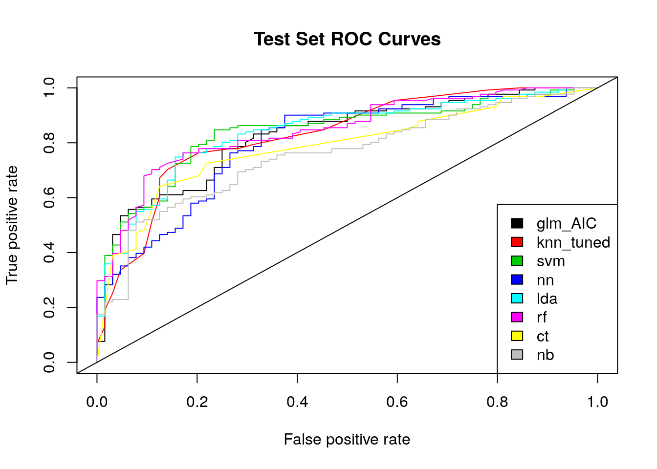
In terms of ROC, we see that the naive bayes model does not achieve the results expected in the first part. According to the curves of the graph, the random forest and the SVM obtain the best results. In order to better interpret these results, we use the area under the ROC curve (AUC). A model is considered good if it obtains an AUC of more than 80%.
#AUC metric
auc <- performance(pred, measure = "auc")
auc <- auc@y.values
auc<- tibble(auc)
auc$model <- c("glm_AIC", "knn_tuned", "svm", "nn", "lda", "rf","ct", "nb")
results_auc <- as.data.frame(lapply(auc, unlist))
results_auc <- results_auc %>% arrange(desc(auc))
results_auc %>% kable() %>% kable_styling()| auc | model |
|---|---|
| 0.8457777 | rf |
| 0.8392176 | svm |
| 0.8377863 | lda |
| 0.8272304 | knn_tuned |
| 0.8268130 | glm_AIC |
| 0.8040315 | nn |
| 0.7858421 | ct |
| 0.7566794 | nb |
best_auc <-
results_auc %>%
  slice_max(auc)

paste("According to the AUC, the best model is", best_auc$model, "with AUC =", round(best_auc$auc, digits = 4)) %>% kable(col.names = NULL, align="l")| According to the AUC, the best model is rf with AUC = 0.8458 |
AUC results confirm the results found with the ROC metric. However, results are totally different from the first part (accuracy metric). It is therefore really difficult to designate the best prediction model.
In order to look beyond these results, we will use the DALEX tool in the next chapter.