Chapter 2 Data understanding and preparation

In this chapter, we will analyse the database in more details in order to be able to build significant prediction models. Moreover, we will look for wrong values among observations and correct them.

Our database is composed of 1,000 observations and contains the following variables:

• obs: observation number
• chk_account: category defining the balance in the checking account in Deutsch Mark (DM)
• duration: loan duration in months
• history: credit history
• new_car: purpose of credit
• used_car: purpose of credit
• furniture: purpose of credit
• radio.tv: purpose of credit
• education: purpose of credit
• retraining: purpose of credit
• amount: credit amount
• sav_acct: category defining the average balance in savings account in DM
• employment: category defining the duration of current employment
• install_rate: installment rate as % of disposable income
• male_div: borrower is a male and divorced
• male_single: borrower is a male and single
• male_mar_or_wid: borrower is a male and married or a male and widower
• co.applicant: borrower has a co-applicant
• guarantor: borrower has a guarantor
• present_resident: category defining the duration of present resident in years
• real_estate: borrower owns real estate
• prop_unkn_none: borrower owns no property
• age: borrower’s age in years
• other_install: borrower has other installment plan credit
• rent: borrower has a rent
• own_res: borrower owns residence
• num_credits: number of existing credits at this bank
• job: category defining the nature of the borrower’s job
• num_dependents: number of people for whom liable to provide maintenance
• telephone: borrower has phone in his or her name
• foreign: borrower is a foreign worker
• risk: borrower’s credit rating is good or bad (response variable)

2.1 Exploratory data analysis (EDA)

We make some cleaning operations in our dataset which is shown below.

german <- read.csv("Data/GermanCredit.csv", sep = ";")

#Renaming OBS. in OBS
colnames(german)[1] <- "OBS"

#Col names in lower case 
colnames(german) <- tolower(colnames(german))

#Creating a new variable in order to know if credit risk is good  (1) or bad (0)
german$risk <- ifelse(german$response == 1, "good", "bad") 
german$risk <- as.factor(german$risk)
#We remove the binary variable response because we will use the caterogical one (risk) that we previously created
german <- german %>% select(-response) 

#Inspecting the data frame, there are numerical and categorical values
datatable(german, rownames=FALSE, fillContainer = TRUE)

2.1.1 Missing values

We check for missing data. No missing data is observed in our database.

missmap(german)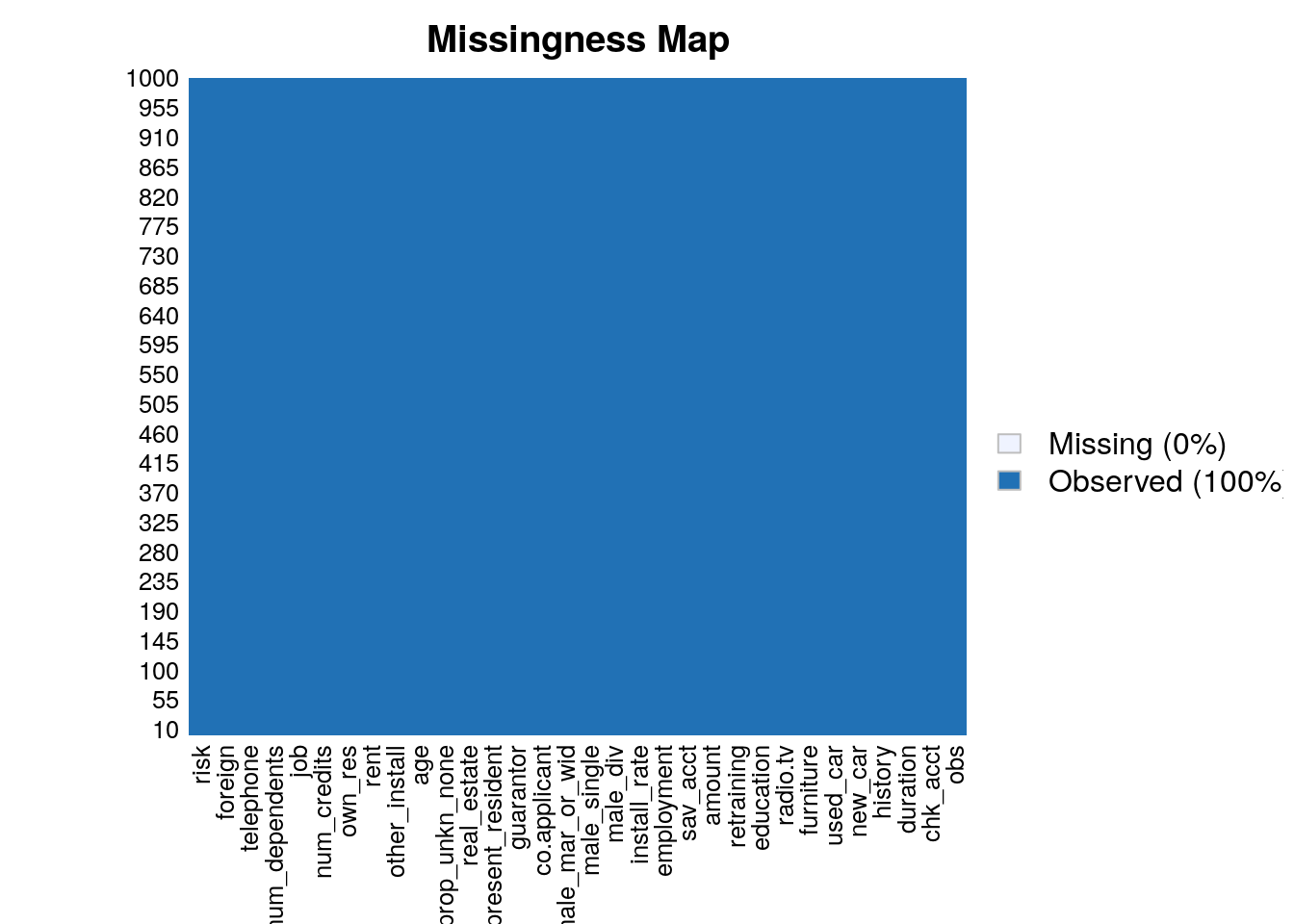

2.1.2 Bad vs Good

Our database is not balanced. There is much more good credits. Therefore, models will tend to predict more often good customers rather than bad ones. We will have to pay attention to the specificity. Nevertheless, data will be balanced in the modeling part.

vs <- inspect_cat(select(german, risk))
show_plot(vs)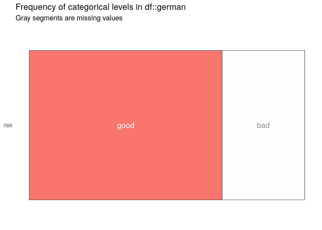

2.1.3 Anomalies

We detected some anomalies in the database:

• guarantor: Max = 2 : It should be 1 instead of 2.
• education: Min = -1 : It should be 1 instead of -1.
• age: Max = 125 : It should be 75 instead of 125 (impossible value).

summary_age<- summary(german$age) %>% round(0) %>% as.data.frame.vector()

summary_education<- summary(german$education) %>% as.data.frame.vector()

summary_guarantor<- summary(german$guarantor) %>% as.data.frame.vector()

summary_duration<- summary(german$duration) %>% round(0) %>% as.data.frame.vector()

summary_chk_acct<- summary(german$chk_acct) %>% as.data.frame.vector()

summary_final <- cbind(summary_age, summary_education, summary_guarantor, summary_duration, summary_chk_acct)
summary_final %>% kable(caption = "Summary", col.names = c("Age", "Education", "Guarantor", "Duration", "Chk_acct"))

Table 2.1: Summary

	Age	Education	Guarantor	Duration	Chk_acct
Min.	19	-1.000	0.000	4	0.000
1st Qu.	27	0.000	0.000	12	0.000
Median	33	0.000	0.000	18	1.000
Mean	36	0.048	0.053	21	1.577
3rd Qu.	42	0.000	0.000	24	3.000
Max.	125	1.000	2.000	72	3.000

We will therefore modify the database with the correct information in order to optimize our future models.

#Data transformation
german$age[537] <- 75
german$education [37] <- 1
german$guarantor [234] <- 1

Also, in order to understand better the variables, we make some modifications in our database but only for the EDA part. Indeed, we rename the job categories as well as the categories of the savings account feature.

german_EDA <- german

german_EDA$job <-
    factor(
        german_EDA$job,
        levels = 0:3,
        labels = c(
            "unemployed/unskilled",
            "unskilled - resident",
            "skilled employee/official",
            "management/self-employed/
highly qualifed employee/officer"
        )
    )

german_EDA$sav_acct <-
    factor(
        german_EDA$sav_acct,
        levels = 0:4,
        labels = c(
            "< 100 DM",
            "100 ≤ ... < 500 DM",
            "500 ≤ ··· < 1000 DM",
            "≥ 1000 DM",
            "unknown/no savings account"
        )
    )

2.1.4 Analysis of the clients

2.1.4.1 Type of jobs

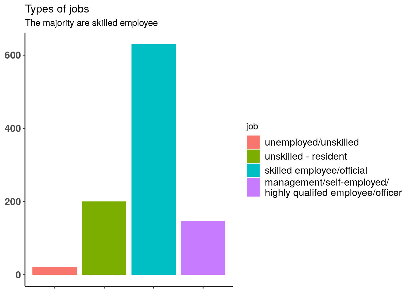
Most of the clients have a qualified job. This variable may play a role in our future predictions.

ggplot(german_EDA, aes(x = job, fill = job)) +
    geom_bar() +
    ggtitle("Types of jobs", subtitle = "The majority are skilled employee") +
    theme_bw() +
    theme(
        axis.text = element_text(size = 12, face = "bold"),
        legend.text = element_text(size = 12),
        axis.title.x = element_blank(),
        axis.title.y = element_blank(),
        panel.grid.major = element_blank(),
        panel.grid.minor = element_blank(),
        panel.border = element_blank(),
        axis.line = element_line(colour = "black"),
        axis.text.x = element_blank()
    )

2.1.4.2 Type of savings account

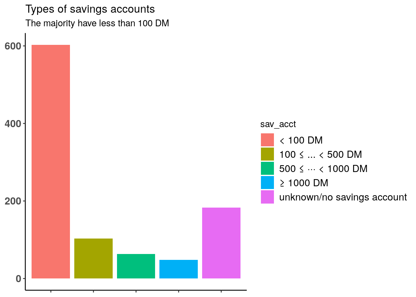
Most customers have less than 100 DM in their account. Indeed, the customer base consists mainly of small savers.

ggplot(german_EDA, aes(x = sav_acct, fill = sav_acct)) +
    geom_bar() +
    ggtitle("Types of savings accounts", subtitle = "The majority have less than 100 DM") +
    theme_bw() +
    theme(
        axis.text = element_text(size = 12, face = "bold"),
        legend.text = element_text(size = 12),
        axis.title.x = element_blank(),
        axis.title.y = element_blank(),
        panel.grid.major = element_blank(),
        panel.grid.minor = element_blank(),
        panel.border = element_blank(),
        axis.line = element_line(colour = "black"),
        axis.text.x = element_blank()
    )

2.1.4.3 Purpose of credit

Below, we display the risk among purpose of credit. Radio TV is the most frequent purpose for a credit and people who borrow money to buy a new car are most often defined as at-risk customers.

purpose<- german_EDA %>% select("new_car", "used_car", "furniture", "radio.tv", "education", "retraining", "risk") 

#new_car
df_new_car_good <- purpose %>% select("new_car", "risk") %>% filter(risk == "good", new_car == 1) %>% count(name = "good")
df_new_car_bad <- purpose %>% select("new_car", "risk") %>% filter(risk == "bad", new_car == 1) %>% count(name = "bad")
results_new_car<- cbind(df_new_car_good, df_new_car_bad) 
rownames(results_new_car)[rownames(results_new_car) == "1"] = "new_car"

#used_car
df_used_car_good <- purpose %>% select("used_car", "risk") %>% filter(risk == "good", used_car == 1) %>% count(name = "good")
df_used_car_bad <- purpose %>% select("used_car", "risk") %>% filter(risk == "bad", used_car == 1) %>% count(name = "bad")
results_used_car <- cbind(df_used_car_good, df_used_car_bad) 
rownames(results_used_car)[rownames(results_used_car) == "1"] = "used_car"

#furniture
df_furniture_good <- purpose %>% select("furniture", "risk") %>% filter(risk == "good", furniture == 1) %>% count(name = "good")
df_furniture_bad <- purpose %>% select("furniture", "risk") %>% filter(risk == "bad", furniture == 1) %>% count(name = "bad")
results_furniture <- cbind(df_furniture_good, df_furniture_bad) 
rownames(results_furniture)[rownames(results_furniture) == "1"] = "furniture"

#radio.tv
df_radio.tv_good <- purpose %>% select("radio.tv", "risk") %>% filter(risk == "good", radio.tv == 1) %>% count(name = "good")
df_radio.tv_bad <- purpose %>% select("radio.tv", "risk") %>% filter(risk == "bad", radio.tv == 1) %>% count(name = "bad")
results_radio.tv <- cbind(df_radio.tv_good, df_radio.tv_bad) 
rownames(results_radio.tv)[rownames(results_radio.tv) == "1"] = "radio.tv"

#education
df_education_good <- purpose %>% select("education", "risk") %>% filter(risk == "good", education == 1) %>% count(name = "good")
df_education_bad <- purpose %>% select("education", "risk") %>% filter(risk == "bad", education == 1) %>% count(name = "bad")
results_education <- cbind(df_education_good, df_education_bad) 
rownames(results_education)[rownames(results_education) == "1"] = "education"

#retraining
df_retraining_good <- purpose %>% select("retraining", "risk") %>% filter(risk == "good", retraining == 1) %>% count(name = "good")
df_retraining_bad <- purpose %>% select("retraining", "risk") %>% filter(risk == "bad", retraining == 1) %>% count(name = "bad")
results_retraining <- cbind(df_retraining_good, df_retraining_bad) 
rownames(results_retraining)[rownames(results_retraining) == "1"] = "retraining"

all_results <- rbind(results_new_car, results_used_car, results_furniture, results_radio.tv, results_education, results_retraining)

results_final <- all_results %>% melt()


results_final <- results_final %>% mutate(purpose = c("new_car", "used_car", "furniture", "radio.tv", "education", "retraining", "new_car", "used_car", "furniture", "radio.tv", "education", "retraining"))

colnames(results_final) <- c("risk", "value", "purpose")


results_final %>%  ggplot(aes(reorder(x = purpose, -value), y = value, fill = risk)) +
  geom_bar(position = 'dodge', stat = 'identity') + theme_bw() +
  theme(
    axis.text = element_text(size = 12, face = "bold"),
    legend.text = element_text(size = 12),
    axis.title.y = element_blank()
  ) +
  ggtitle("Risk analysis by purpose of credit", subtitle = "Radio TV is the most frequent purpose for a credit") + xlab('Purpose of credit')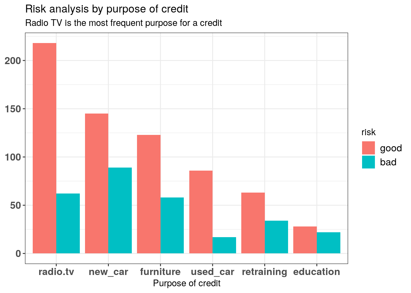 

2.1.4.4 Gender analysis

Most of the customers are men. We note, however, that the probability of being at risk among women is high. It will therefore be interesting to take gender into account during the construction of our models.

#Create a variable sex 
german_EDA <- german_EDA %>% mutate(sex = ifelse(male_div == 1 | male_single == 1 | male_mar_or_wid == 1, 1,0))

german_EDA$sex <-
    factor(german_EDA$sex,
           levels = 0:1,
           labels = c("female",
                      "male"))


german_EDA %>% select(sex, risk) %>% group_by(sex, risk) %>% count() %>%
    ggplot(aes(x = sex, y = n, fill = risk)) +
    geom_bar(position = 'dodge', stat = 'identity') +
    geom_text(aes(label = n),
              position = position_dodge(width = 0.9),
              vjust = -0.25) +
    ggtitle("Risk analysis by gender", subtitle = "The data set is not well balanced")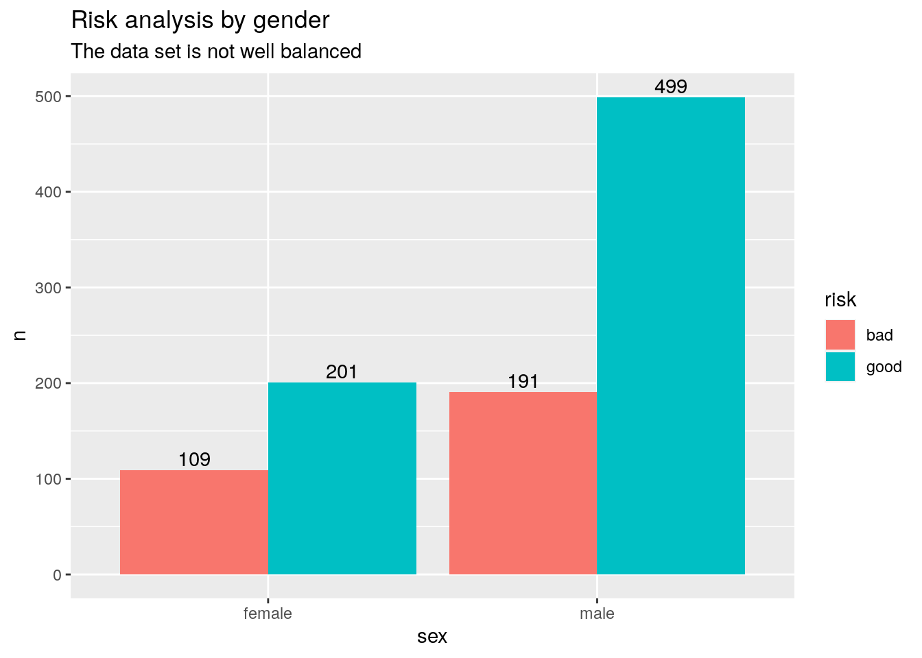

2.1.5 Boxplot - variable explanation

duration: At-risk clients have longer credit duration.

amount: The median amounts are slightly higher for the at-risk category.

age: The median for good payers is higher.

b1 <- german %>% ggplot(aes(x = risk, y = duration)) +
    geom_boxplot(
        outlier.colour = "red",
        outlier.shape = 8,
        outlier.size = 1
    ) 

b2 <- german %>% ggplot(aes(x = risk, y = amount)) +
    geom_boxplot(
        outlier.colour = "red",
        outlier.shape = 8,
        outlier.size = 1
    )  
  
b3 <- german %>% ggplot(aes(x = risk, y = age)) +
    geom_boxplot(
        outlier.colour = "red",
        outlier.shape = 8,
        outlier.size = 1
    )

grid.arrange(b1, b2, b3, nrow=1,
             top = textGrob("Box Plot analysis", gp=gpar(fontsize=15, font=2)))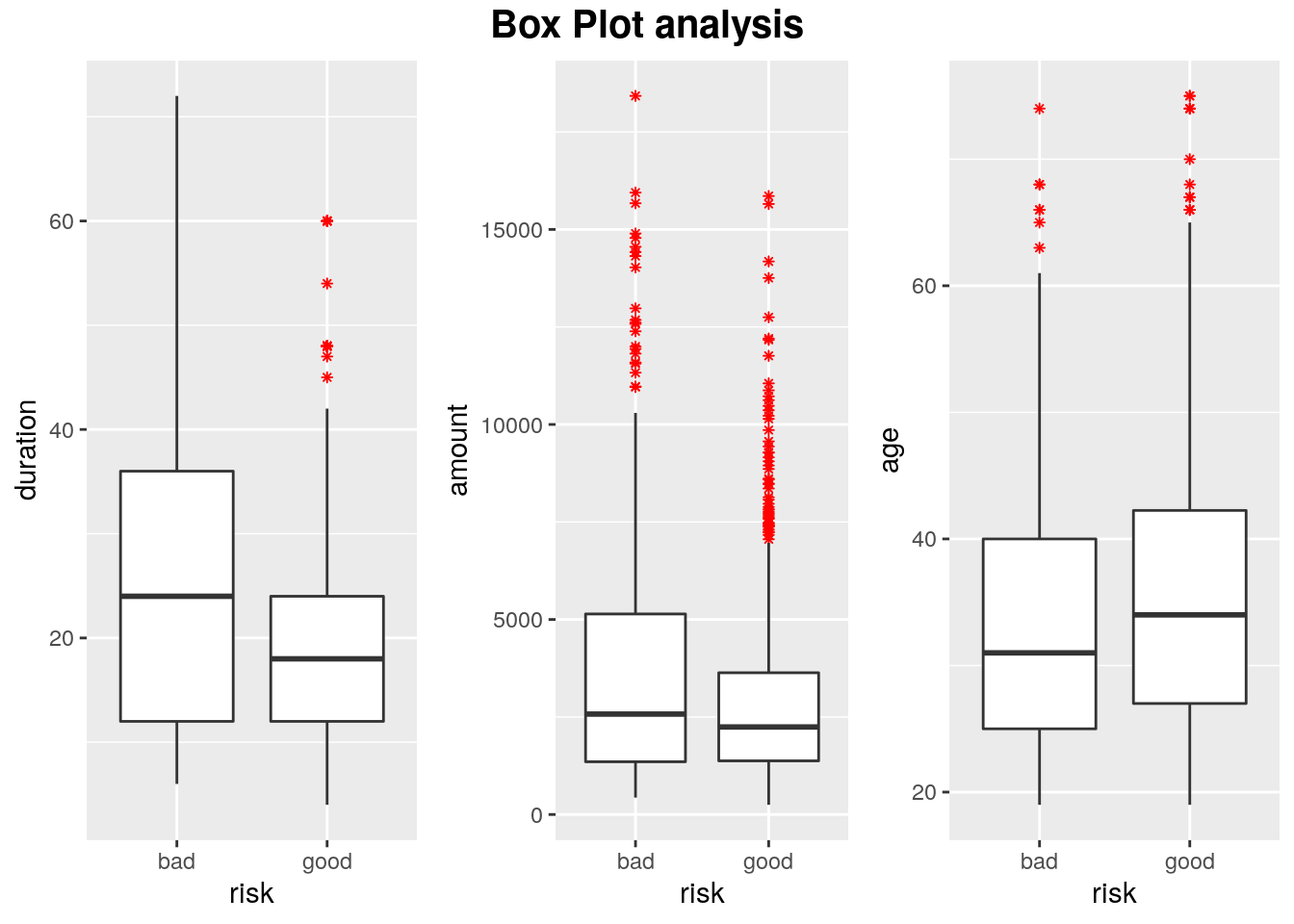

Below, we remark that variables age, amount and duration are right skewed. In order to modify it, we use the log transformation to change them into a normal distribution.

g1 <-  ggplot(german, aes(x = age)) + 
  geom_histogram(bins = 20, fill = 'pink', colour = 'black') + 
  ggtitle('Age distribution') + 
  xlab('Age') +
  ylab('Frequency')

g2 <- ggplot(german, aes(x = amount)) + 
  geom_histogram(bins = 20, fill = 'turquoise', colour = 'black') + 
  ggtitle('Amount distribution') + 
  xlab('Credit_Amount') +
  ylab('Frequency')

g3 <- ggplot(german, aes(x = duration)) + 
  geom_histogram(bins = 20, fill = 'lightgoldenrod', colour = 'black') + 
  ggtitle('Duration distribution') + 
  xlab('Duration') +
  ylab('Frequency')

grid.arrange(g1, g2, g3, nrow=1)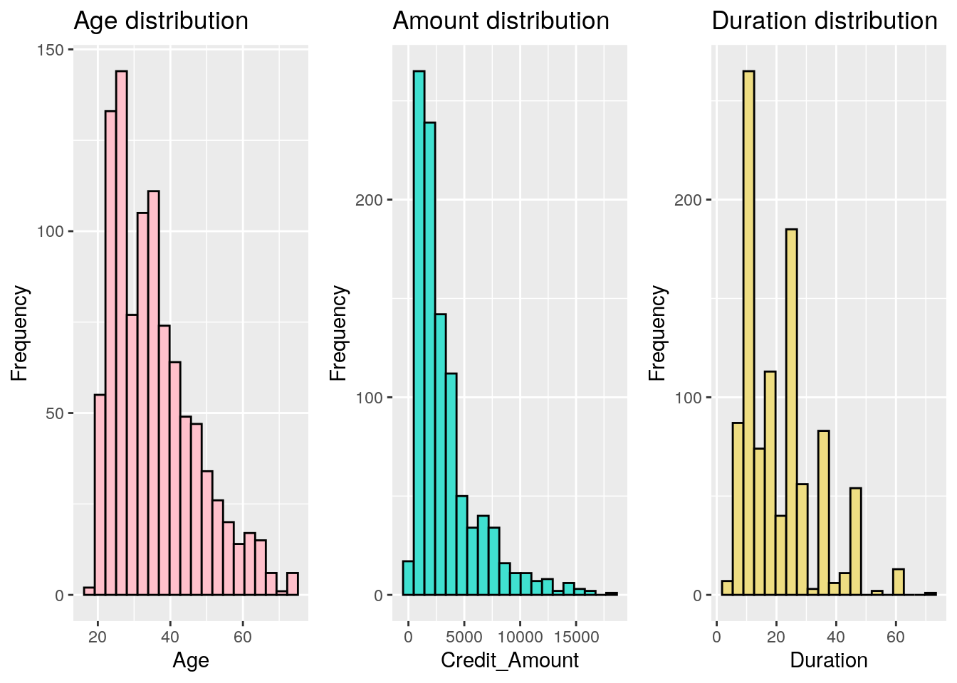

Even if age is still a bit right skewed, it is much better than before as we can see with the following plot. This modification is important in order to guarantee the good reliability of our models.

#Transforming variables
g1 <-  ggplot(german, aes(x = log1p(age))) + 
  geom_histogram(bins = 20, fill = 'pink', colour = 'black') + 
  ggtitle('Age distribution') + 
  xlab('Age') +
  ylab('Frequency')

g2 <- ggplot(german, aes(x = log1p(amount))) + 
  geom_histogram(bins = 20, fill = 'turquoise', colour = 'black') + 
  ggtitle('Amount distribution') + 
  xlab('Credit_Amount') +
  ylab('Frequency')

g3 <- ggplot(german, aes(x = log1p(duration))) + 
  geom_histogram(bins = 20, fill = 'lightgoldenrod', colour = 'black') + 
  ggtitle('Duration distribution') + 
  xlab('Duration') +
  ylab('Frequency')


grid.arrange(g1, g2, g3, nrow=1)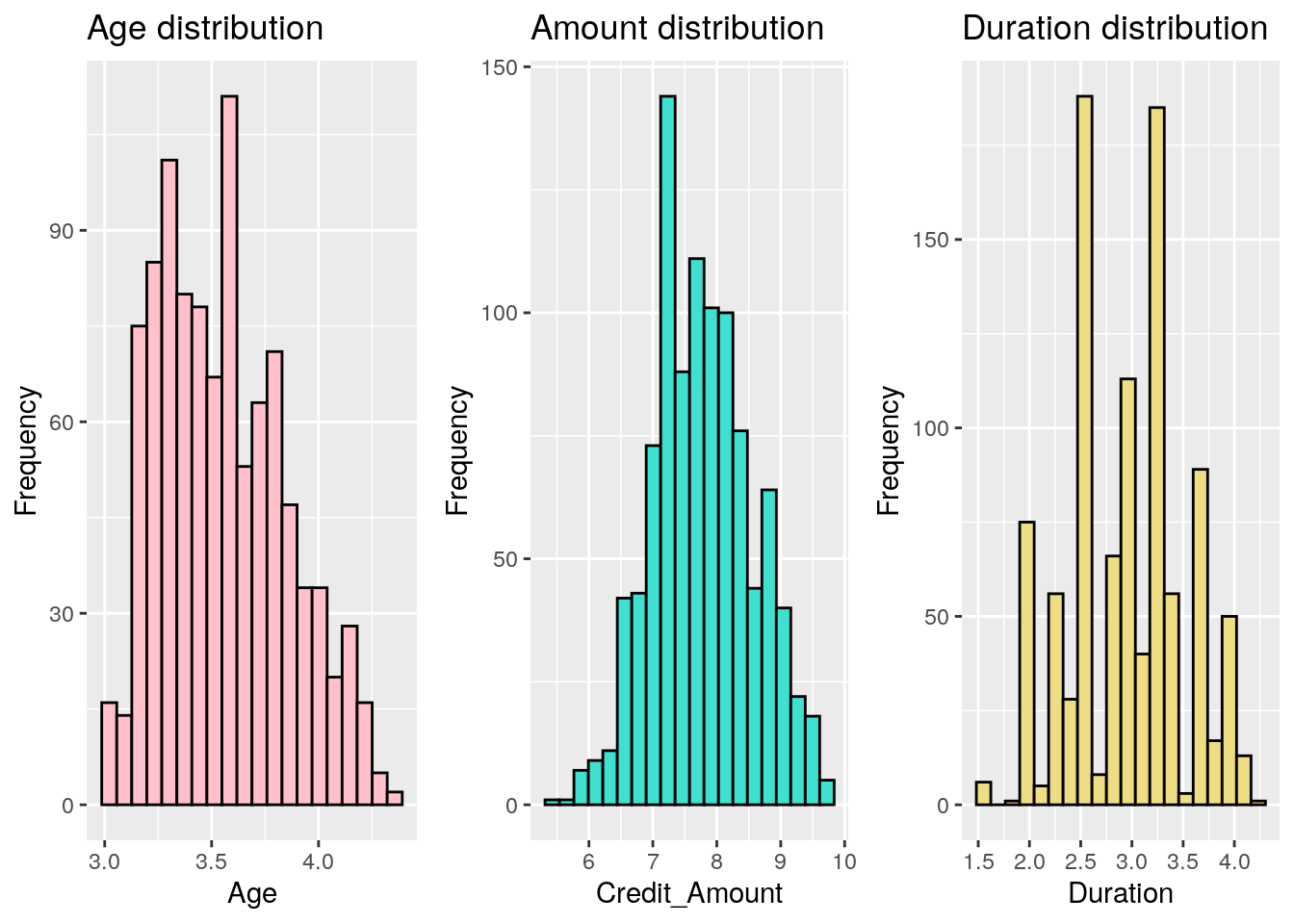

2.1.6 Correlation

Correlation for risk = good: There is a correlation between amount and duration. This makes sense.

correlation_good <- german %>% filter(risk == "good") %>% select(amount, age, duration) 

ggpairs(correlation_good)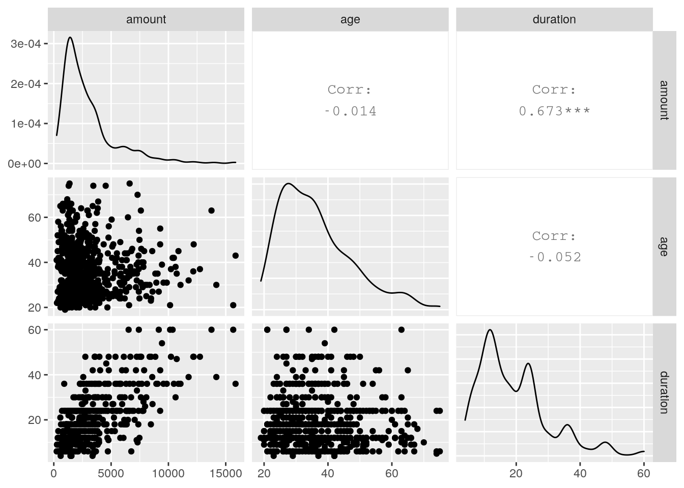

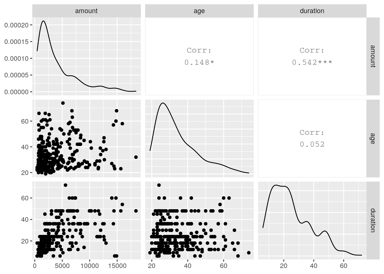
Correlation for risk = bad: The amount is correlated with the duration of the contract and somewhat with the age of the person.

correlation_bad <- german %>% filter(risk == "bad") %>% select(amount, age, duration) 

ggpairs(correlation_bad)