Chapter 4 DALEX
The DALEX method is useful to better understand the models that we are using. Some models used in the previous part were complex. Accuracy and ROC are therefore not enough to really know what is going on behind the models. It is therefore difficult to choose among models.
This method will bring us new knowledge on the database and on the importance and behavior of certain variables.
In order to carry out this analysis, we relied on the book Explanatory Model Analysis (Burzykowski (2020)).
To begin, we use the balanced training set and the test set from the modeling part.
We decided to explain the following interesting models:
- Random forest
- Logistic regression
- Nearest neighbour classification (KNN)
- Linear discriminant analysis (LDA)
- Neural network
The analysis using the DALEX method is carried out in four phases:
- Training the models with metric set as “accuracy”
- Prepare an explainer
- Dataset level
- Instance level
4.1 Training the models
This part consists in creating the models we are going to compare. To do this, we base ourselves on existing models from modeling part (accuracy metric).
train_control <- trainControl(method = "cv", number = 5)
metric <- "Accuracy"

#random forest model
hp_rf <- expand.grid(.mtry = (1:15))
set.seed(531)
fit_rf <- train(
  risk ~ .,
  data = german.tr.bal,
  method = 'rf',
  metric = metric,
  trControl = train_control,
  tuneGrid = hp_rf
)

#glm model
set.seed(123)
fit_glm_AIC = train(
  form = risk ~ chk_acct + history + used_car + education + sav_acct + employment + male_single +
  prop_unkn_none + rent + job + foreign + Log1pDurationstd,
  data = german.tr.bal,
  trControl = train_control,
  method = "glmStepAIC",
  metric = metric,
  family = "binomial"
)

#knn model
set.seed(456)
fit_knn_tuned = train(
  risk ~ .,
  data = german.tr.bal,
  method = "knn",
  metric = metric,
  trControl = train_control,
  tuneGrid = expand.grid(k = seq(1, 101, by = 1))
)

#LDA
set.seed(1839)
fit_LDA <- train(risk ~ .,
                 data = german.tr.bal,
                 method = "lda",
                 metric = metric,
                 trControl = train_control)

#Neural network
hp_nn <- expand.grid(size = 2:10,
                     decay = seq(0, 0.5, 0.05))
set.seed(2006)
fit_nn <- train(
  form = risk ~ .,
  data = german.tr.bal,
  trControl = train_control,
  tuneGrid = hp_nn,
  method = "nnet",
  metric = metric
)
4.2 Create an explainer
The explainer function allows us to explain a single feature of a model. The data collected on our different models will be the basis to generate explanatory graphs.
#Transform the variable to predict into numeric values
german.te <- transform(german.te, risk=as.numeric(as.factor(german.te$risk))-1)

#random forest model
explainer_rf <- DALEX::explain(fit_rf,
                        data = german.te[,-28],
                        y = german.te$risk,
                        label = "Random Forest")

#glm model
explainer_glm <- DALEX::explain(fit_glm_AIC,
                        data = german.te[,-28],
                        y = german.te$risk,
                        label = "Logistic regression")

#knn model
explainer_knn <- DALEX::explain(fit_knn_tuned,
                        data = german.te[,-28],
                        y = german.te$risk,
                        label = "KNN")

#lda model
explainer_lda <- DALEX::explain(fit_LDA,
                        data = german.te[,-28],
                        y = german.te$risk,
                        label = "LDA")

#nn model
explainer_nn <- DALEX::explain(fit_nn,
                        data = german.te[,-28],
                        y = german.te$risk,
                        label = "Neural network")
4.3 Dataset level
Here, we will analyse the predictions with a dataset level.
4.3.1 Model performance and model diagnostic
Because we already computed the accuracy and the ROC of each model in the previous part, we will not reproduce the results here. We will rather display the distributions of the residuals. Usually, in a good model, residuals deviate randomly from zero. Therefore, we should observe a symmetric distribution around zero (mean = 0). In addition, we want to limit the variability of residuals in our models, therefore we aim to have residuals close to zero.
4.3.1.1 Distribution of the residuals
#random forest model
rf_hist <- DALEX::model_performance(explainer_rf)

#glm model
glm_hist <- DALEX::model_performance(explainer_glm)

#knn model
knn_hist <- DALEX::model_performance(explainer_knn)

#lda model
lda_hist <- DALEX::model_performance(explainer_lda)

#neural network model
nn_hist <- DALEX::model_performance(explainer_nn)

plot(rf_hist, glm_hist, knn_hist, lda_hist, nn_hist, geom = "histogram")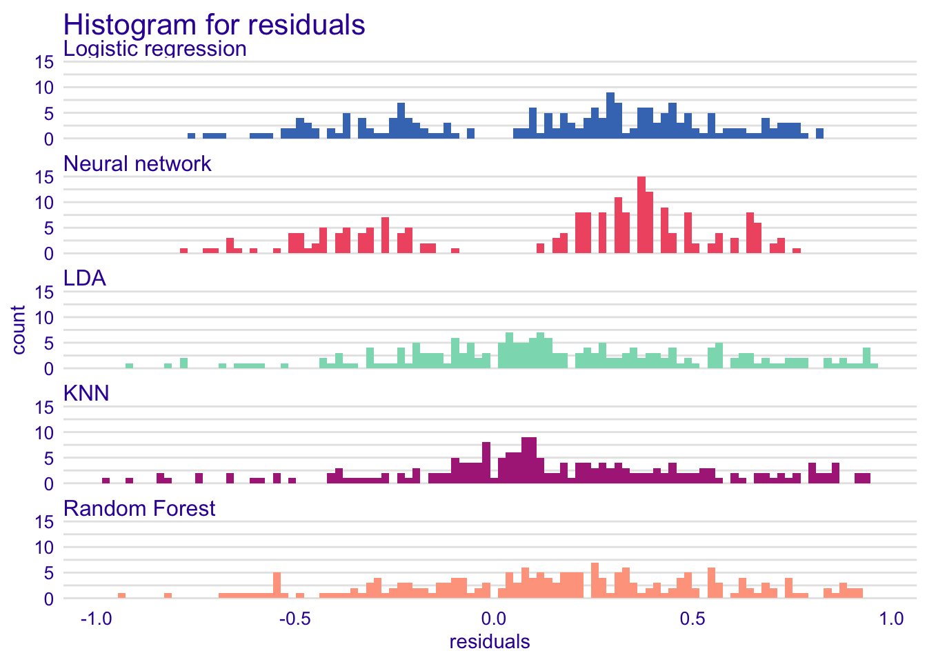
In the histograms, we can see that KNN, LDA and ranfom forest models have residuals closer to zero than for the logistic regression and the neural network model. Residuals are also randomly distributed. We have a bimodal distribution as we want to classify the observations between two groups (good credit and bad credit). The bimodal distribution is more evident for the logistic regression and the neural network. The distribution of the LDA, KNN and random forest is more spreaded than for logistic regression and neural network.
Overall, the residual distribution of our models is a bit skewed to the right.
rf_bp <- DALEX::model_performance(explainer_rf)
glm_bp <- DALEX::model_performance(explainer_glm)
knn_bp <- DALEX::model_performance(explainer_knn)
lda_bp <- DALEX::model_performance(explainer_lda)
nn_bp <- DALEX::model_performance(explainer_nn)

plot(rf_bp, glm_bp, knn_bp, lda_bp, nn_bp, geom = "boxplot")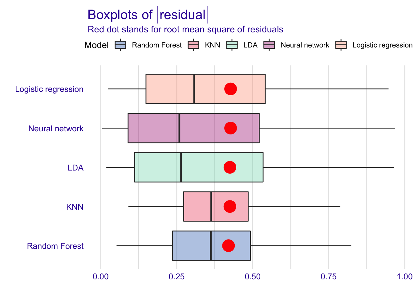
The box-and-whisker plots of the residuals confirm the results and show that LDA residuals are more frequently close to zero with neural network, but also more spreaded.
Residuals and observed values
A perfect predictive model would have residuals on the horizontal line. But, a good model has residuals around the horizontal line showing random deviations between observed and predicted values.
When comparing the residuals versus the observed values, we see that KNN model have less values of residuals close to zero unlike other models.
rfdiag <- explainer_rf %>% model_diagnostics() %>% plot(variable = "y", yvariable = "residuals", smooth = FALSE)
glmdiag <- explainer_glm %>% model_diagnostics() %>% plot(variable = "y", yvariable = "residuals", smooth = FALSE)
knndiag <- explainer_knn%>% model_diagnostics() %>% plot(variable = "y", yvariable = "residuals", smooth = FALSE)
ldadiag <- explainer_lda%>% model_diagnostics() %>% plot(variable = "y", yvariable = "residuals", smooth = FALSE)
nndiag <- explainer_nn%>% model_diagnostics() %>% plot(variable = "y", yvariable = "residuals", smooth = FALSE)

grid.arrange(rfdiag, glmdiag, knndiag, ldadiag, nndiag, nrow = 2)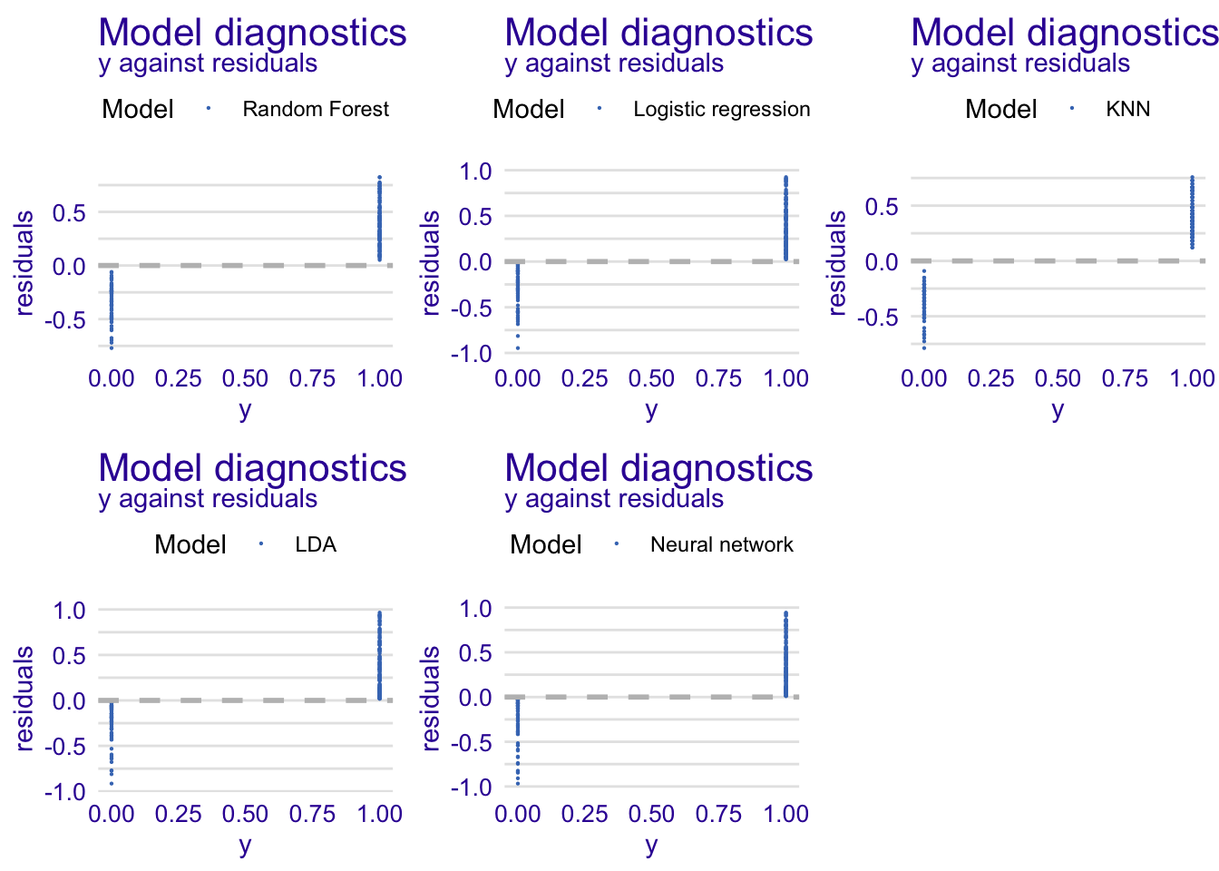
Predicted and observed values
Below, we display the predicted values versus the observed ones.
rfdiag1 <- explainer_rf %>% model_diagnostics() %>% plot(variable = "y", yvariable = "y_hat", smooth = FALSE)
glmdiag1 <- explainer_glm %>% model_diagnostics() %>% plot(variable = "y", yvariable = "y_hat", smooth = FALSE)
knndiag1 <- explainer_knn%>% model_diagnostics() %>% plot(variable = "y", yvariable = "y_hat", smooth = FALSE)
ldadiag1 <- explainer_lda%>% model_diagnostics() %>% plot(variable = "y", yvariable = "y_hat", smooth = FALSE)
nndiag1 <- explainer_nn%>% model_diagnostics() %>% plot(variable = "y", yvariable = "y_hat", smooth = FALSE)

grid.arrange(rfdiag1, glmdiag1, knndiag1,ldadiag1, nndiag1, nrow = 2)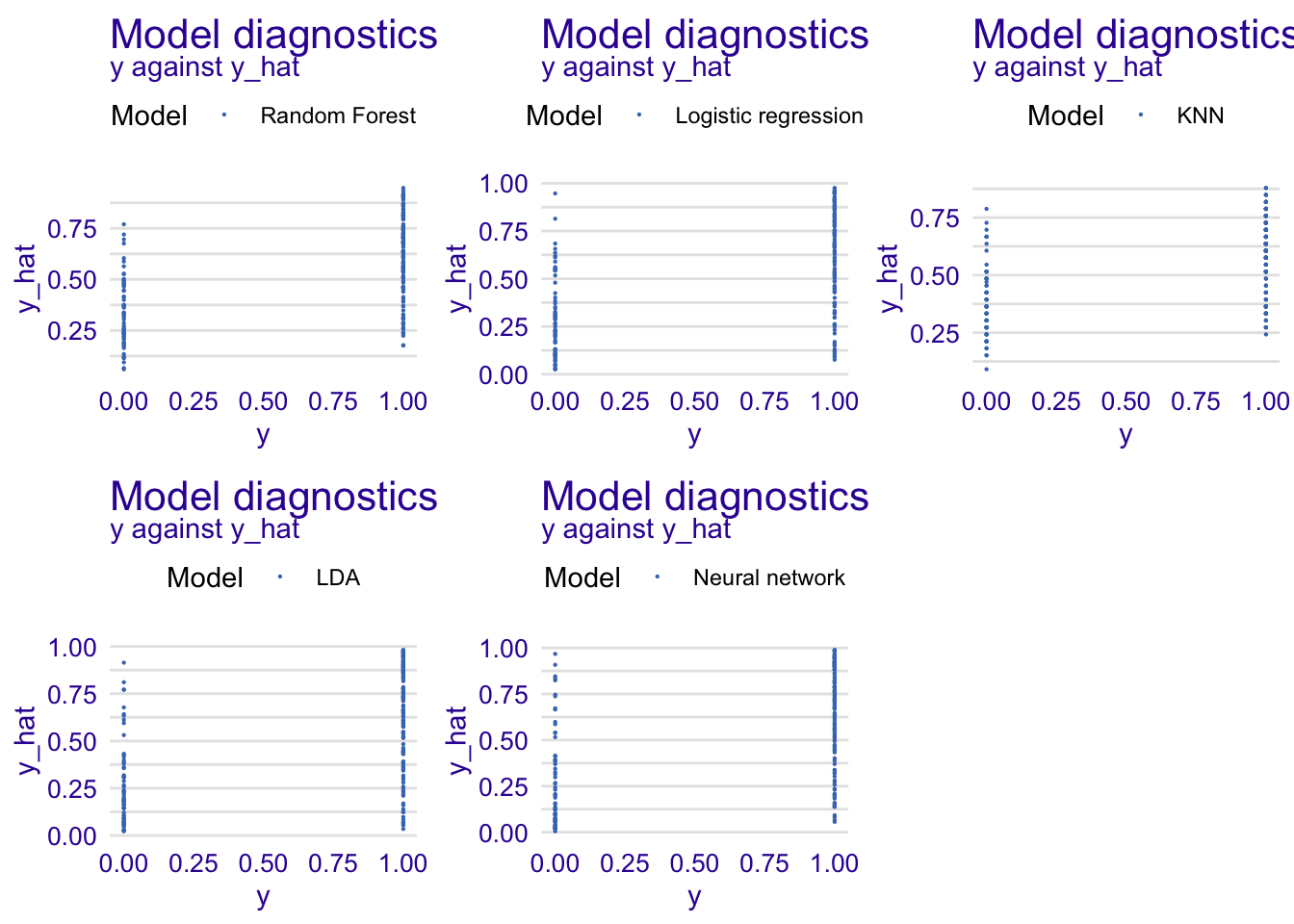
Index of residuals
We do not see any pattern among residuals which show that residuals as randomly distributed around zero. Again, we remark that KNN model have less residual values around zero which is not really good.
rfdiag2 <- explainer_rf %>% model_diagnostics() %>% plot(variable = "ids", yvariable = "residuals", smooth = FALSE)
glmdiag2 <- explainer_glm %>% model_diagnostics() %>% plot(variable = "ids", yvariable = "residuals", smooth = FALSE)
knndiag2 <- explainer_knn%>% model_diagnostics() %>% plot(variable = "ids", yvariable = "residuals", smooth = FALSE)
ldadiag2 <- explainer_lda%>% model_diagnostics() %>% plot(variable = "ids", yvariable = "residuals", smooth = FALSE)
nndiag2 <- explainer_nn%>% model_diagnostics() %>% plot(variable = "ids", yvariable = "residuals", smooth = FALSE)

grid.arrange(rfdiag2, glmdiag2, knndiag2, ldadiag2, nndiag2, nrow = 2)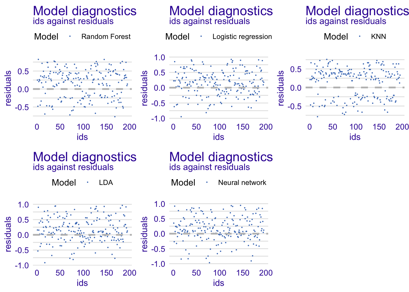
4.3.2 Model parts
This part is essential to know the importance ouf our variables in our models. We will use six important variables of each model and analyse them.
4.3.2.1 Random forest model
explainer_rf %>% model_parts() %>% plot(show_boxplots = FALSE) + ggtitle("Feature Importance ", "")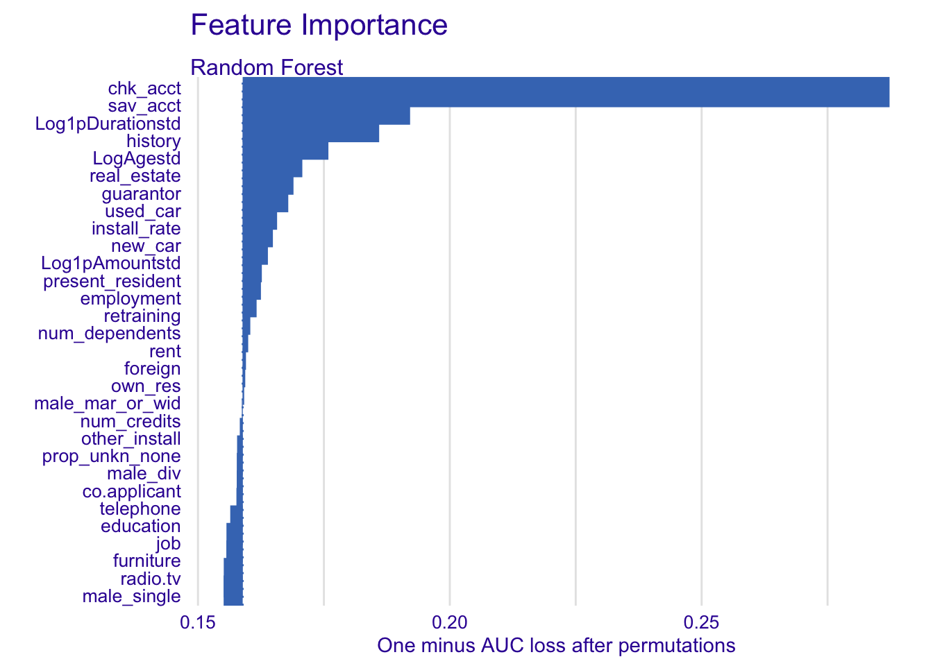
In our random forest model, we select the following variables :
- chk_acct
- Log1pDurationstd
- history
- sav_acct
- Log1pAmountstd
- guarantor
4.3.2.2 Logistic regression model
explainer_glm %>% model_parts() %>% plot(show_boxplots = FALSE) + ggtitle("Feature Importance ", "")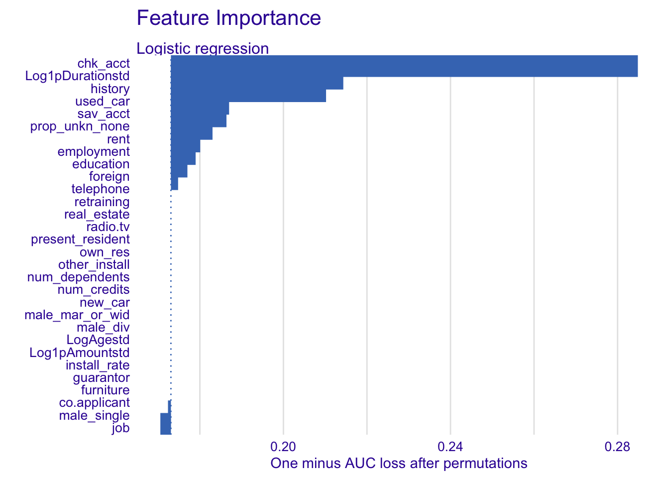
For the logistic regression, we will use:
- chk_acct
- history
- Log1pDurationstd
- sav_acct
- education
- used_car
4.3.2.3 Nearest neighbour classification (KNN)
explainer_knn %>% model_parts() %>% plot(show_boxplots = FALSE) + ggtitle("Feature Importance ", "")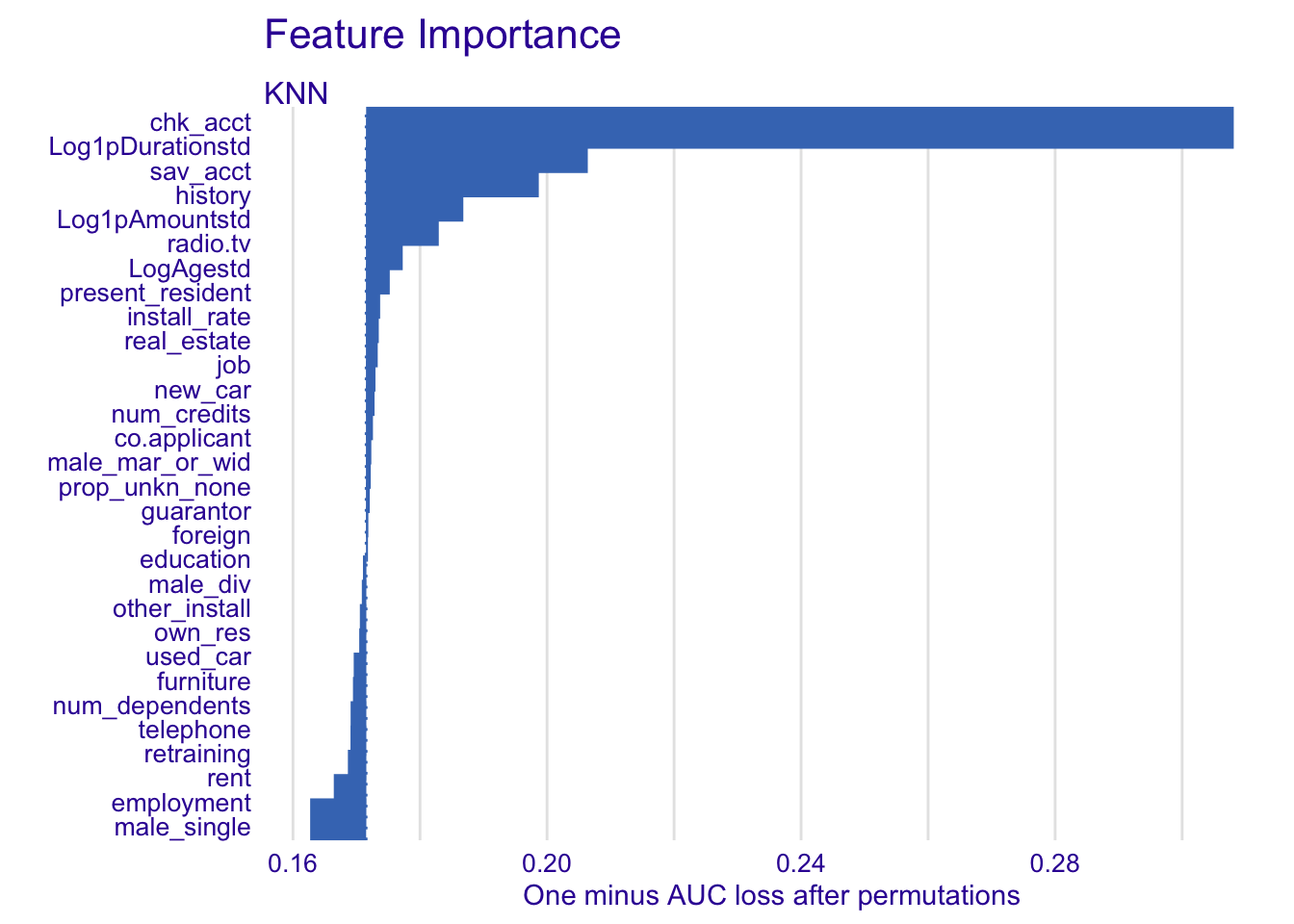
For the KNN model:
- chk_acct
- Log1pDurationstd
- sav_acct
- history
- LogAgestd
- Log1pAmountstd
4.3.2.4 Linear discriminant analysis (LDA)
explainer_lda %>% model_parts() %>% plot(show_boxplots = FALSE) + ggtitle("Feature Importance ", "")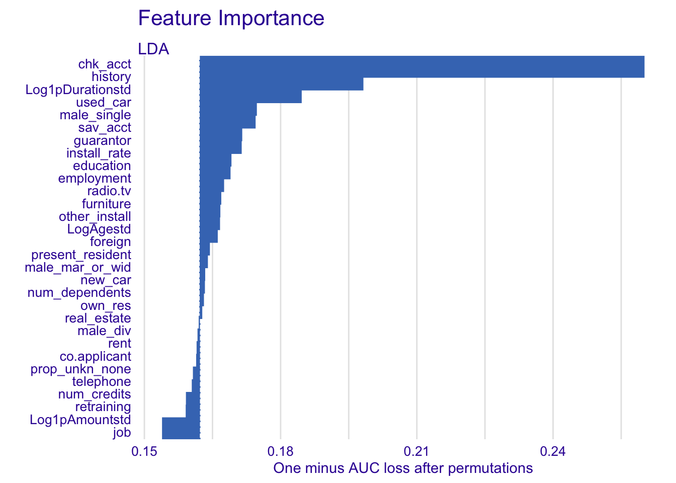
For LDA:
- chk_acct
- history
- Log1pDurationstd
- sav_acct
- guarantor
- used_car
4.3.2.5 Neural network
explainer_nn %>% model_parts() %>% plot(show_boxplots = FALSE) + ggtitle("Feature Importance ", "")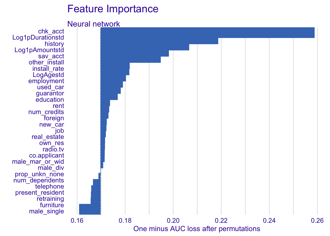
For neural network:
- chk_acct
- Log1pDurationstd
- history
- sav_acct
- Log1pAmountstd
- install_rate
4.3.3 Model profile
In this part, we look for the profile of the important numerical variables of each model.
4.3.3.1 Random forest model
model_profile_rf1 <- model_profile(explainer_rf, type = "partial", variables = c("sav_acct", "chk_acct", "Log1pDurationstd", "history", "Log1pAmountstd", "guarantor"))

plot(model_profile_rf1, variables = c("sav_acct", "chk_acct", "Log1pDurationstd", "history", "Log1pAmountstd", "guarantor")) + ggtitle("Partial dependence profile ", "")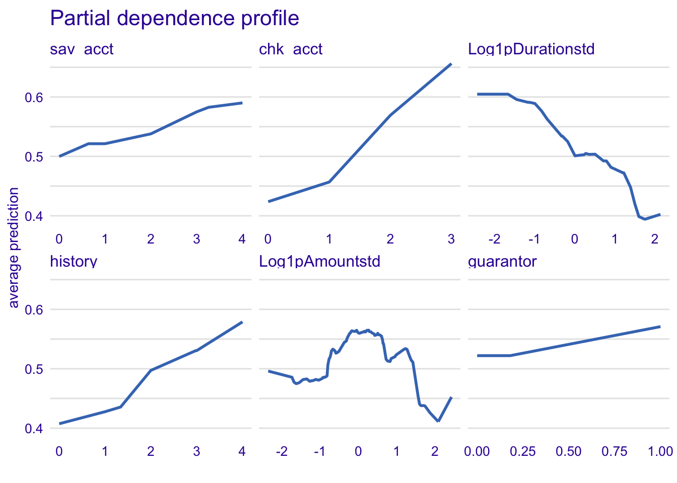
The more your have money on the savings account, the more likely you will be classified as a good credit. It is the same trend for the checking account variable. Reciprocally, the longer the log credit period increases (Log1pDurationstd), the less likely the customer will be defined as good credit. The variable Log1pAmountstd is difficult to interpret.
4.3.3.2 Logistic regression model
model_profile_glm1 <- model_profile(explainer_glm, type = "partial", variables = c("chk_acct", "Log1pDurationstd", "sav_acct", "history", "education", "used_car"))

plot(model_profile_glm1, variables = c("chk_acct", "Log1pDurationstd", "sav_acct", "history", "education", "used_car"))  + ggtitle("Partial dependence profile ", "")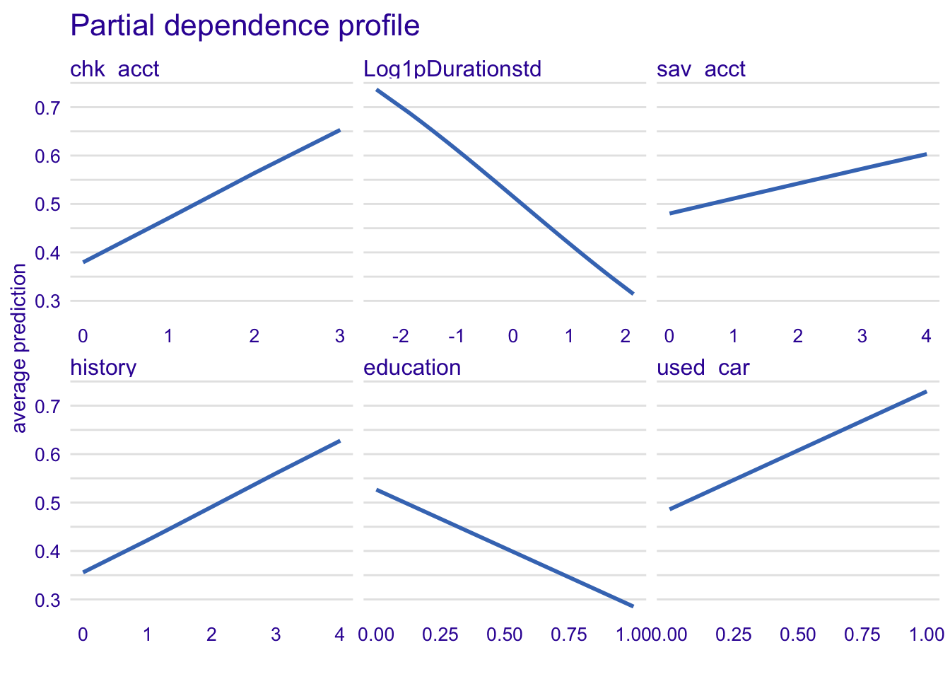
The longer is the credit duration of a customer, the less risky he is for a credit. Here, we can see with history variable that the more critical is the account, the more likely is the classification as good credit risk which is quite not realistic. Also, if the customer has no education, he is more likely to be classified as a good credit risk. Finally, if the borrower wants a credit to buy a used card, he has more chance to be classifed as good.
4.3.3.3 Nearest neighbour classification (KNN)
model_profile_knn1 <- model_profile(explainer_knn, type = "partial", variables = c("sav_acct", "chk_acct", "Log1pDurationstd", "history", "Log1pAmountstd", "LogAgestd"))

plot(model_profile_knn1, variables = c("sav_acct", "chk_acct", "Log1pDurationstd", "history", "Log1pAmountstd", "LogAgestd")) + ggtitle("Partial dependence profile ", "")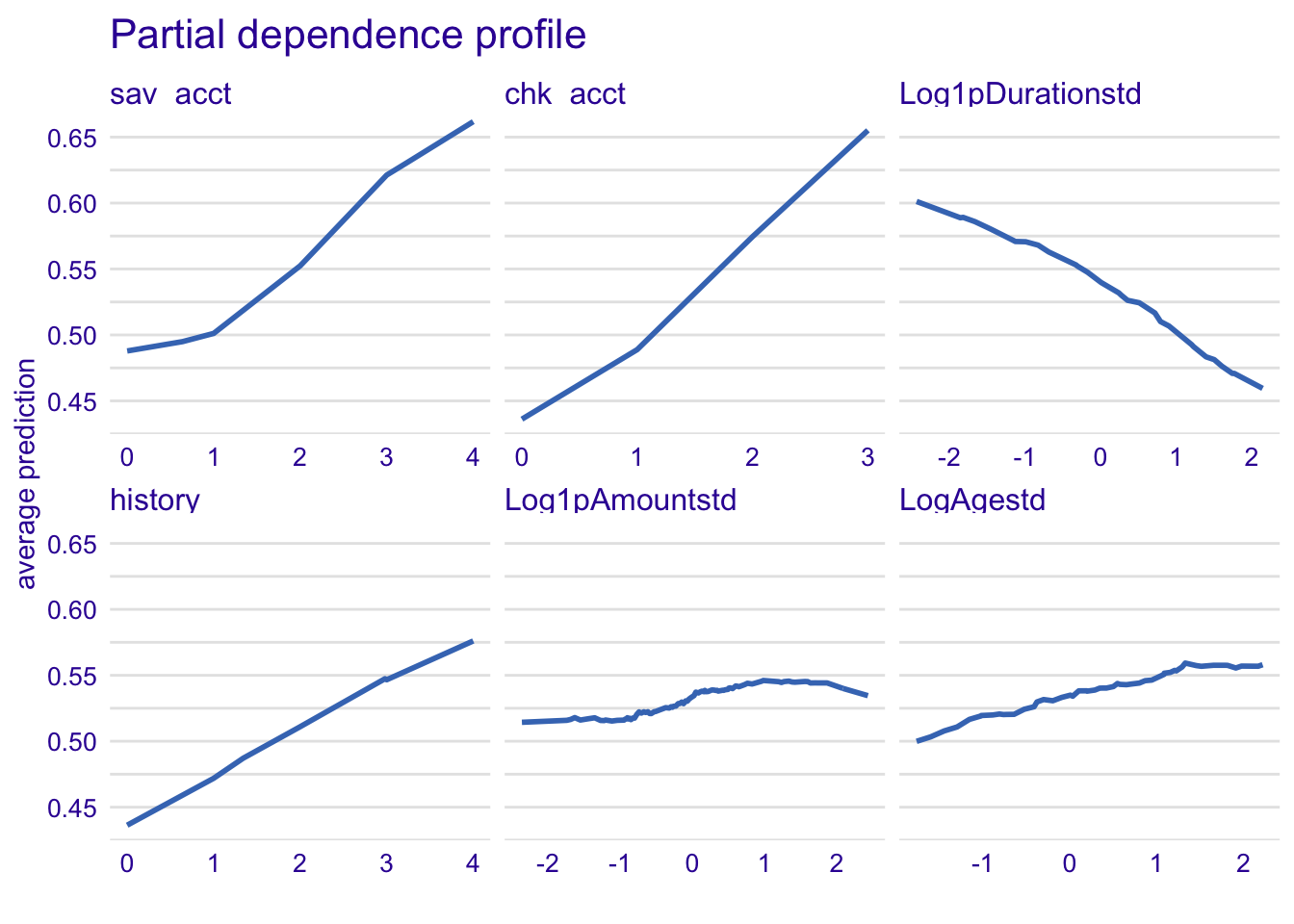
The relationship of sav_acct and chk_acct is even stronger with KNN model.
4.3.3.4 Linear discriminant analysis (LDA)
model_profile_knn1 <- model_profile(explainer_knn, type = "partial", variables = c("sav_acct", "chk_acct", "Log1pDurationstd", "history", "guarantor", "used_car"))

plot(model_profile_knn1, variables = c("sav_acct", "chk_acct", "Log1pDurationstd", "history", "guarantor", "used_car"))  + ggtitle("Partial dependence profile ", "")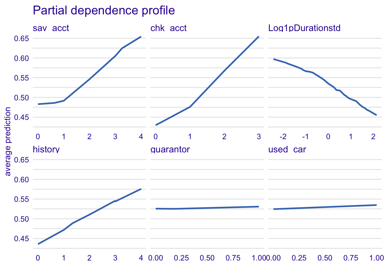
With LDA, there is the same effect than with previous models except for the variable used_car.
4.3.3.5 Neural network
model_profile_knn1 <- model_profile(explainer_knn, type = "partial", variables = c("sav_acct", "chk_acct", "Log1pDurationstd", "history", "Log1pAmountstd", "install_rate"))

plot(model_profile_knn1, variables = c("sav_acct", "chk_acct", "Log1pDurationstd", "history", "Log1pAmountstd", "install_rate")) + ggtitle("Partial dependence profile ", "")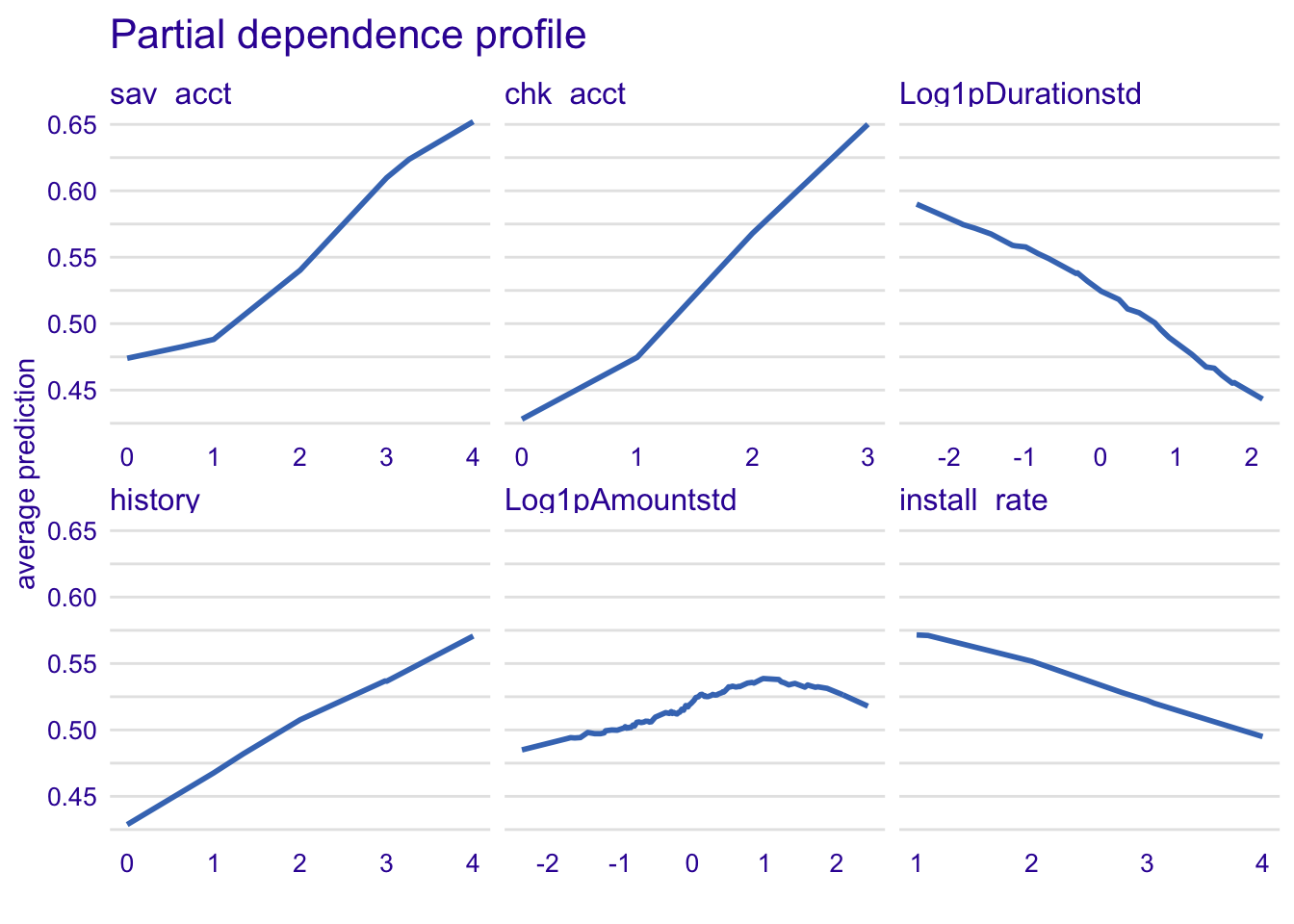
For the variable intall_rate, the more percentage of installment rate as percentage of disposable income, the less likely is the customer to be classified as good credit risk.
Common important variables between models
- chk_acct
- Log1pDurationstd
- sav_acct
- history
#Compare models with common important variables
model_profile_rf_com <- model_profile(explainer_rf, variables = c("chk_acct", "Log1pDurationstd", "sav_acct", "history"))
model_profile_glm_com <- model_profile(explainer_glm, variables = c("chk_acct", "Log1pDurationstd", "sav_acct", "history"))
model_profile_knn_com <- model_profile(explainer_knn, variables = c("chk_acct", "Log1pDurationstd", "sav_acct", "history"))
model_profile_lda_com <- model_profile(explainer_lda, variables = c("chk_acct", "Log1pDurationstd", "sav_acct", "history"))
model_profile_nn_com <- model_profile(explainer_nn, variables = c("chk_acct", "Log1pDurationstd", "sav_acct", "history"))

plot(model_profile_rf_com, model_profile_glm_com, model_profile_knn_com, model_profile_lda_com, model_profile_nn_com, variables = c("chk_acct", "Log1pDurationstd", "sav_acct", "history")) + ggtitle("Partial dependence profile", "")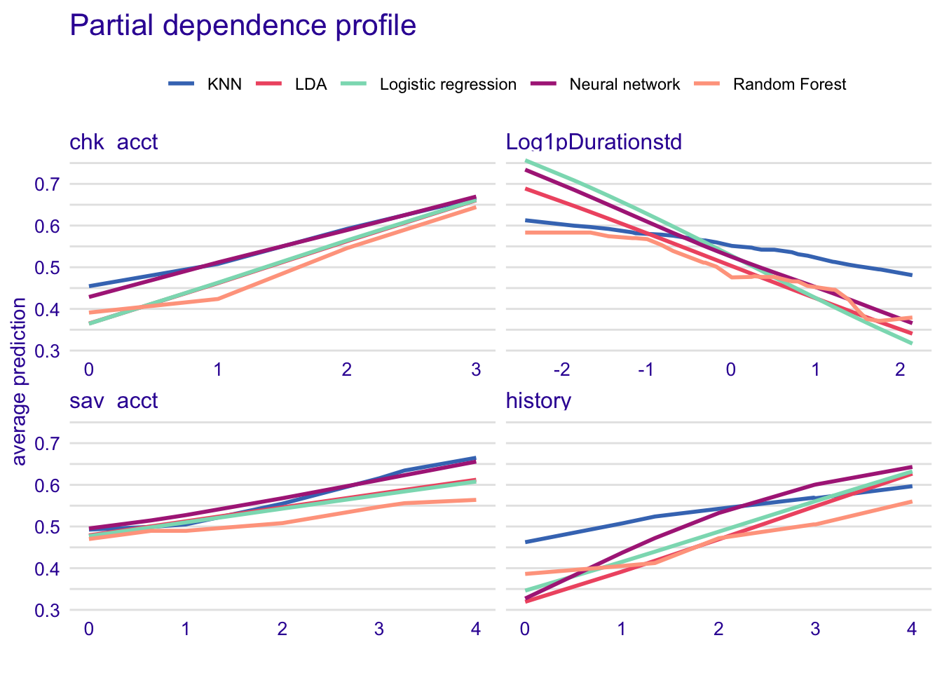
The KNN model does not capture the effect of the Log1pDurationstd when predicting the model. Moreover, KNN seems to overestimate the effet of the history variable on the dependent variable and the LDA model seems to underestimate it. Chk_acct and sav_acct effects are well captured by each model. Therefore, they are very important variables to predict the good or bad credit.
4.4 Instance level
#The instance we want to analyze (the 5th row)
single_customer <- german[5,]
4.4.1 Prediction parts
The break down profiles show the variations in the mean predictions. The plots are useful to assess the contribution of each variable to the prediction of the instance. Therefore, we look for changes in the predictions when values of variables are fixed.
Each explanatory variable is describing the instance we want to analyse. The following plots are summarizing the variations in the mean predictions when chk_acct is fixed to 0, male_single to 1, save_acct to 0, etc.
The intercept value corresponds to the mean value of predictions for the complete dataset. The following values show the changes in the mean prediction when values of variables are fixed. The prediction line in purple corresponds to the value of the prediction of the specific instance, it is the sum of the overall mean value and the variations. The green bars and the red ones show respectively the positive and the negative changes in the mean prediction.
4.4.1.1 Random forest model
#Random forest
explainer_rf %>% predict_parts(new_observation = single_customer) %>% plot()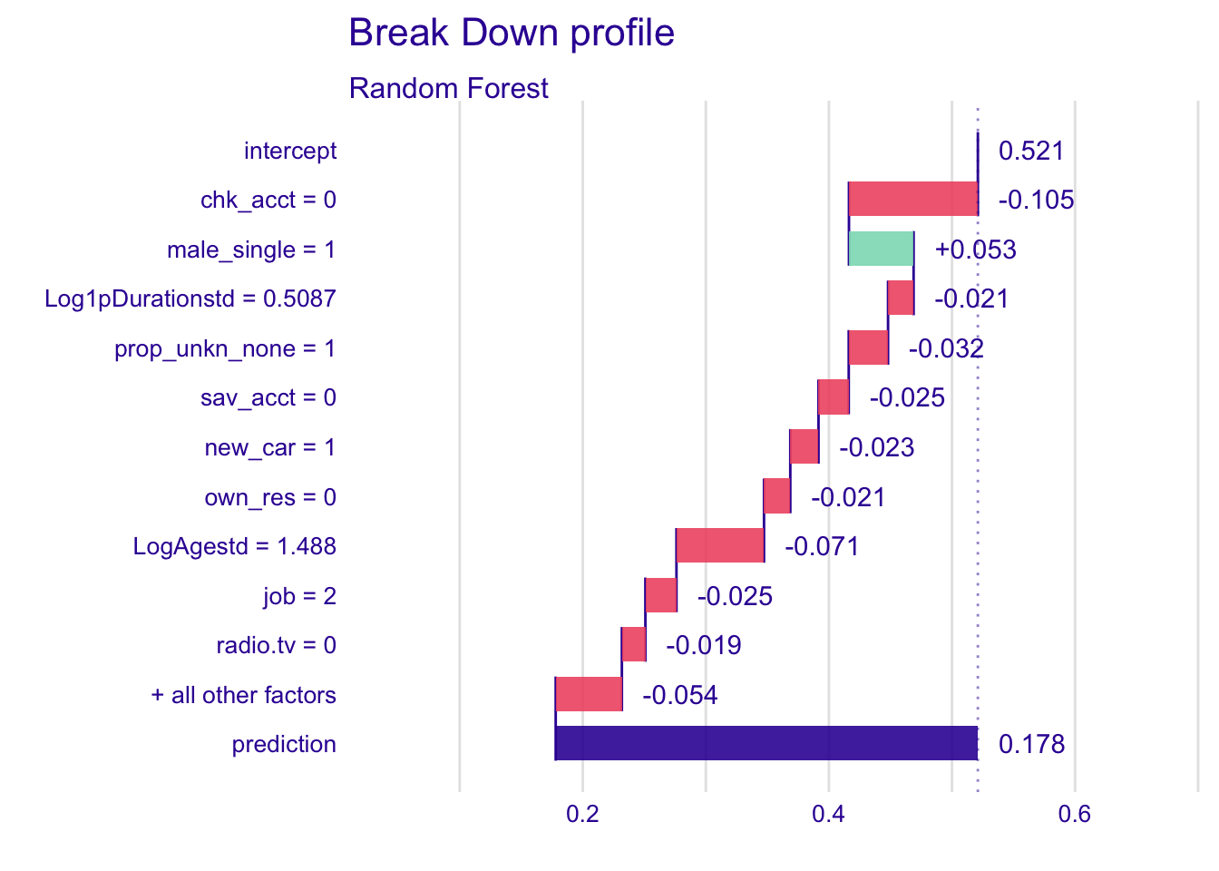
Only the variable male_single has a positive variation in the mean prediction, while others have a negative variation. Chk_acct is the explanatory variable that influences the most the prediction of the instance. By fixing the chk_acct value to 0, we reduce the mean prediction.
4.4.1.2 Logistic regression model
#Logistic regression
explainer_glm %>% predict_parts(new_observation = single_customer) %>% plot()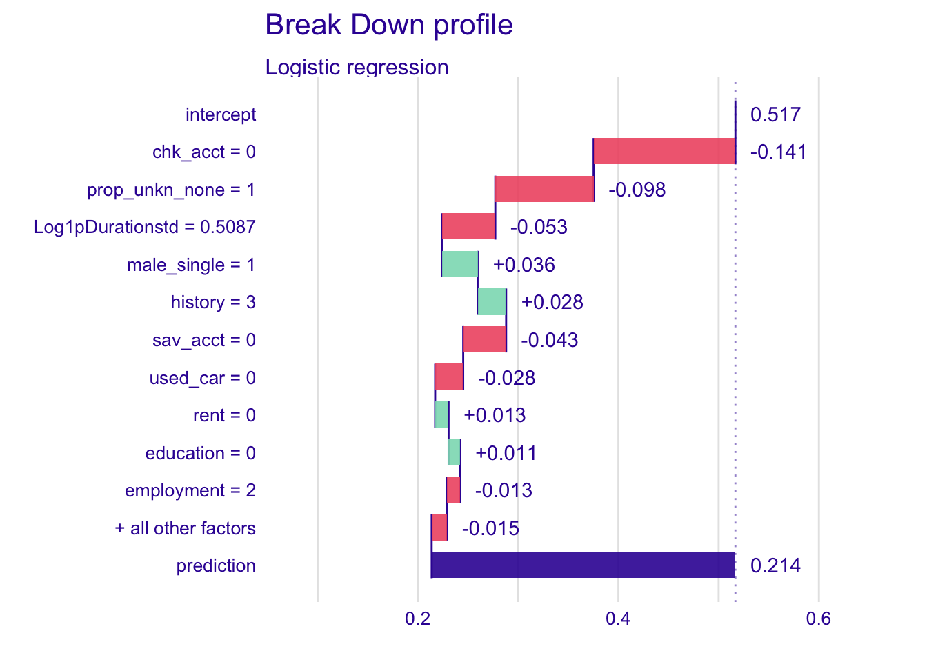
For the logistic regression, more variables have a positive variation on the mean prediction than in the random forest model. The variable chk_acct has the most negative change and influences the most the prediction. Besides chk_acct and prop_unkn_none, other variables have smaller effects on the mean prediction. It could be because they are not important for the prediction or because they effect are closer to the mean of the predictions for this specific instance.
4.4.1.3 Nearest neighbour classification (KNN)
#KNN
explainer_knn %>% predict_parts(new_observation = single_customer) %>% plot()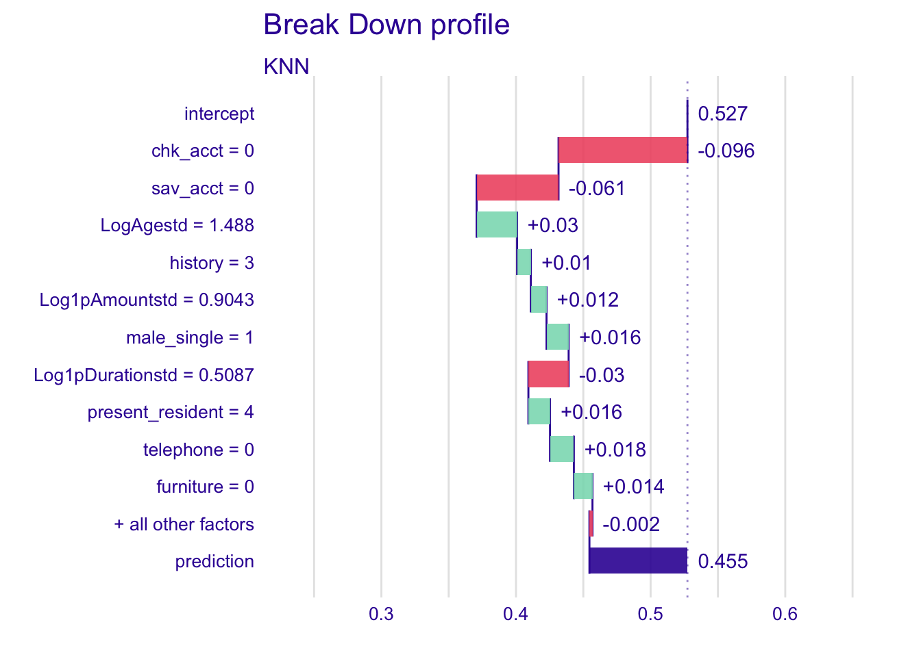
For the KNN model, we have more positive changes in the mean prediction, but chk_acct has still the most important variation, which is a negative one again.
4.4.1.4 Linear discriminant analysis (LDA)
#LDA
explainer_lda %>% predict_parts(new_observation = single_customer) %>% plot()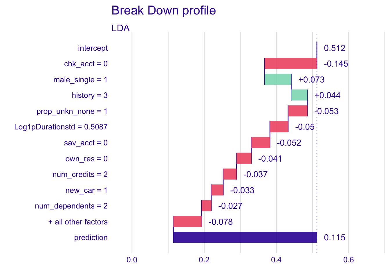
Here, sav_acct has less variation that in the KNN model.
4.4.1.5 Neural network
explainer_nn %>% predict_parts(new_observation = single_customer) %>% plot()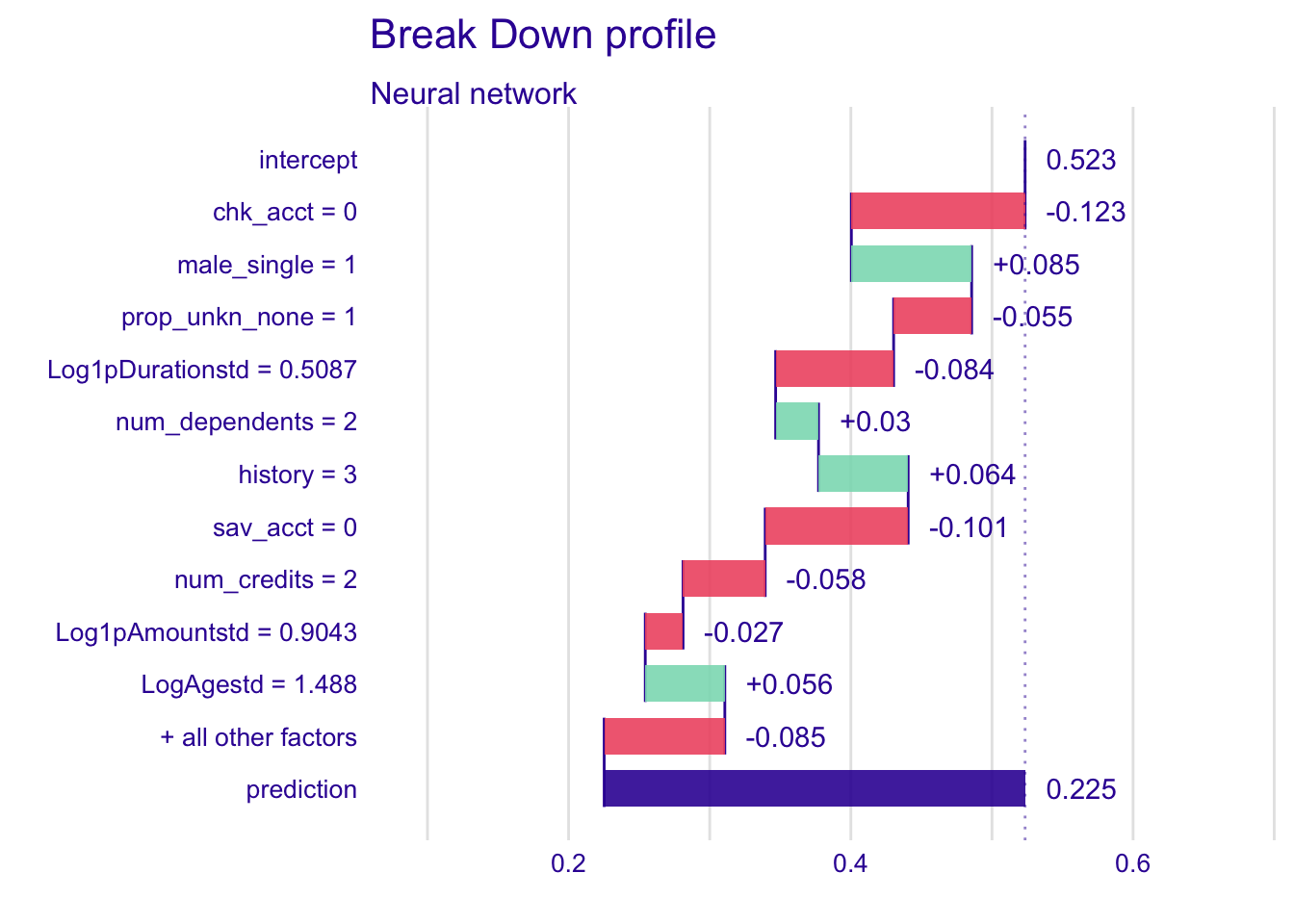
Male_single and history have important positive variations while chk_acct and sav_acct have large negative changes.
4.4.2 Prediction profile
Important variables have a curve with much variation. With the analyse of the profile, we know the role of each variable in the prediction of the instance.
We display a plot for each model representing important numerical variables.
The blue points on the following plots indicate the value of the prediction of the single instance.
4.4.2.1 Random forest model
explainer_rf %>% predict_profile(new_observation = single_customer) %>% plot(
  variables = c(
    "chk_acct",
    "Log1pDurationstd",
    "sav_acct",
    "guarantor", "history", "Log1pAmountstd"
  )
) + ggtitle("Ceteris-paribus profile", "")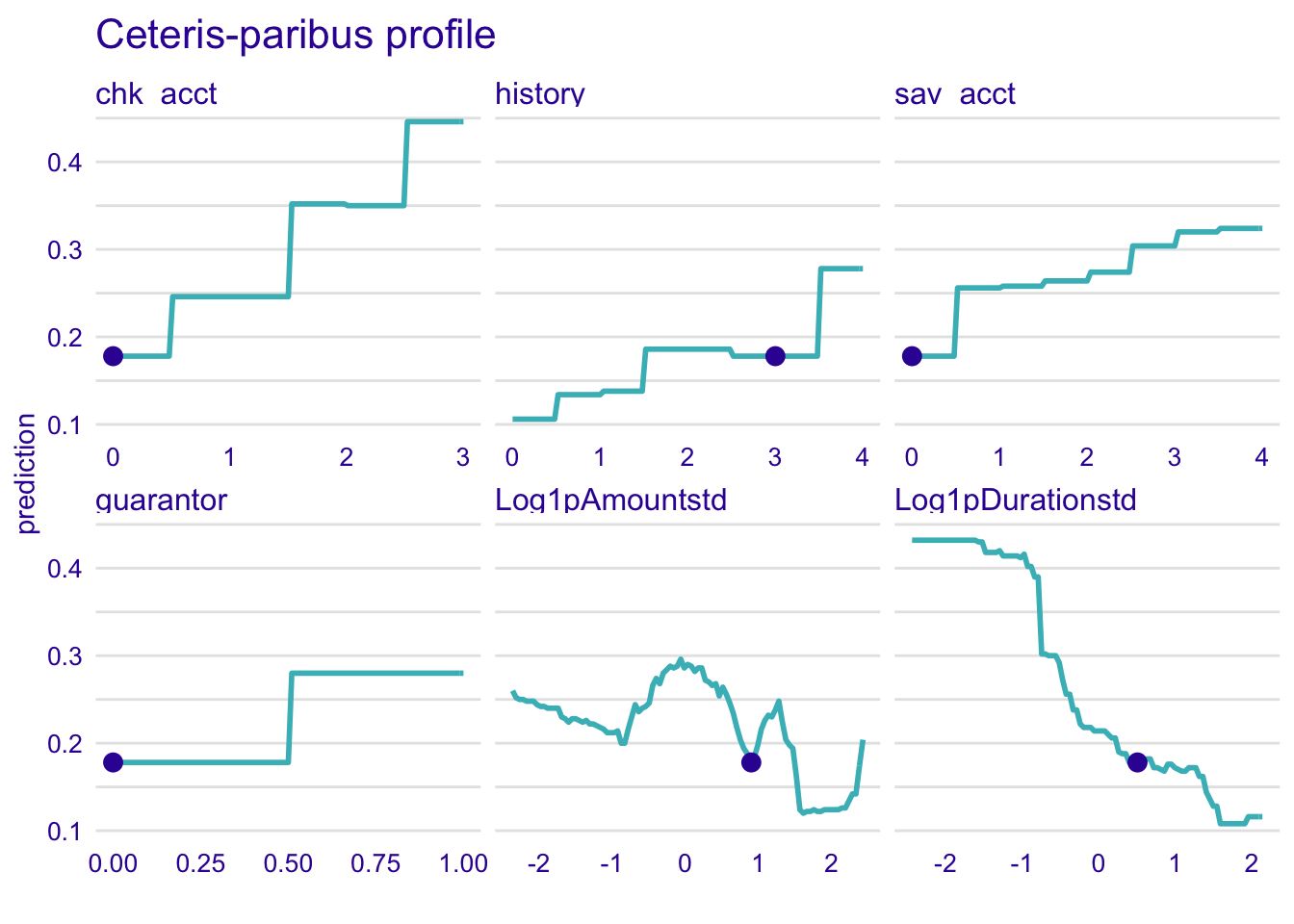
We remark that the profile for the random forest model is a step function.
Here, the higher is the average balance in savings (sav_acct), the richer is the customer and the most likely he will be classified as good credit. His predicted good credit risk probability will increase by more than 10% if he has more than 1,000 DM on his savings account.
For our specific instance, if the customer has a guarantor, he will be most likely classified as a good credit. Here, the observed customer has no guarantor and he is classified as bad credit.
4.4.2.2 Logistic regression model
explainer_glm %>% predict_profile(new_observation = single_customer) %>% plot(
  variables = c(
    "chk_acct",
    "Log1pDurationstd",
    "sav_acct",
    "history", "education", "used_car"
  )
) + ggtitle("Ceteris-paribus profile", "")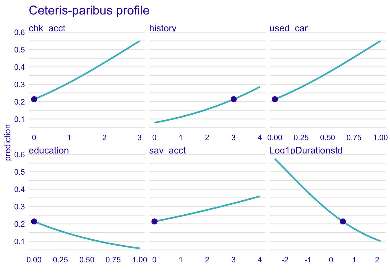
The profile of the logistic regression is smooth unlike for the random forest model.
The more time lasts the credit, the less likely the customer will be classified as a good credit risk.
Here, the customer has no education, therefore he is more likely to be classified as good credit which is strange.
4.4.2.3 Nearest neighbour classification (KNN)
explainer_knn %>% predict_profile(new_observation = single_customer) %>% plot(
  variables = c(
    "chk_acct",
    "Log1pDurationstd",
    "sav_acct",
    "Log1pAmountstd", "history", "LogAgestd"
  )
) + ggtitle("Ceteris-paribus profile", "")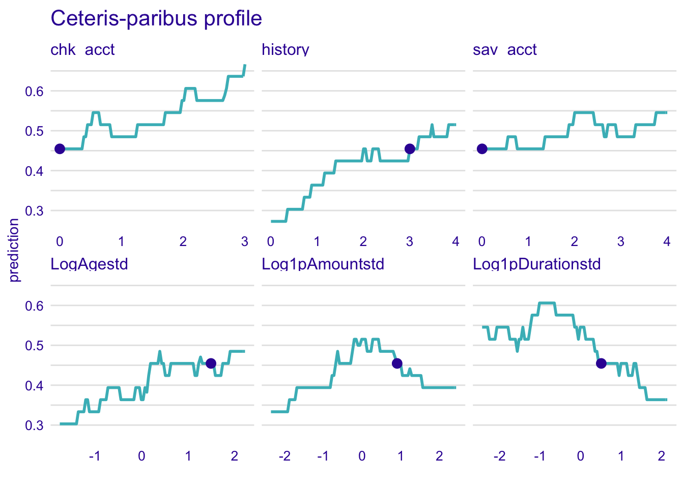
For KNN, there is much more variability and curves are not smooth. Therefore it is more complicated to interpret the results. The trend for the sav_acct is less obvious than in other models.
4.4.2.4 Linear discriminant analysis (LDA)
explainer_lda %>% predict_profile(new_observation = single_customer) %>% plot(
  variables = c(
    "chk_acct",
    "Log1pDurationstd",
    "sav_acct",
    "guarantor",
    "used_car", "history"
  )
) + ggtitle("Ceteris-paribus profile", "")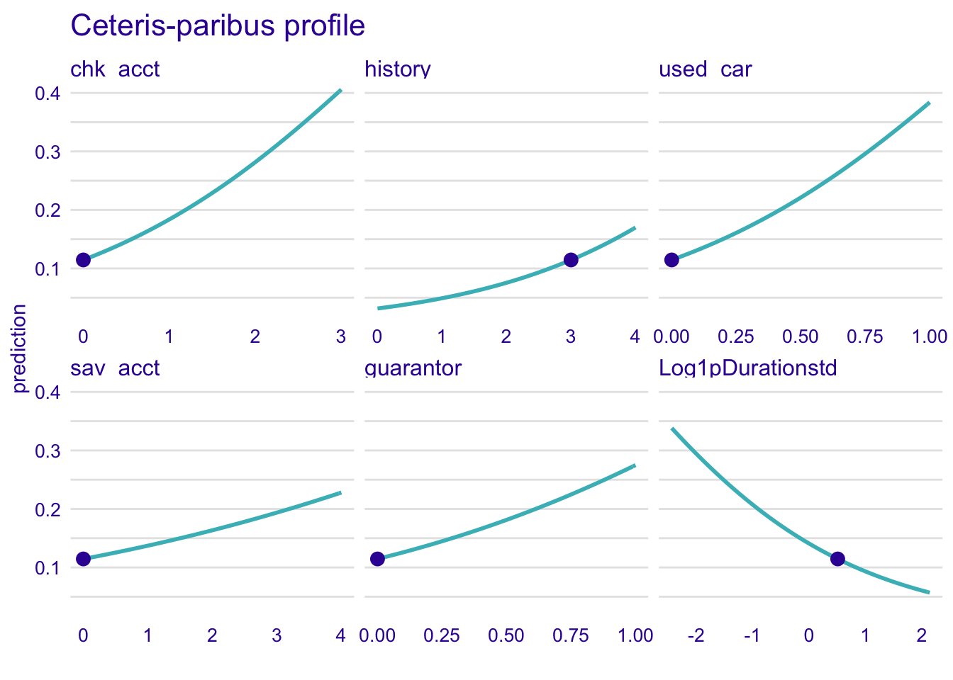
The effect is really obvious for chk_acct, used_car and Log1pDurationstd.
4.4.2.5 Neural network
explainer_nn %>% predict_profile(new_observation = single_customer) %>% plot(
  variables = c(
    "chk_acct",
    "Log1pDurationstd",
    "sav_acct",
    "install_rate",
    "Log1pAmountstd", "history"
  )
) + ggtitle("Ceteris-paribus profile", "")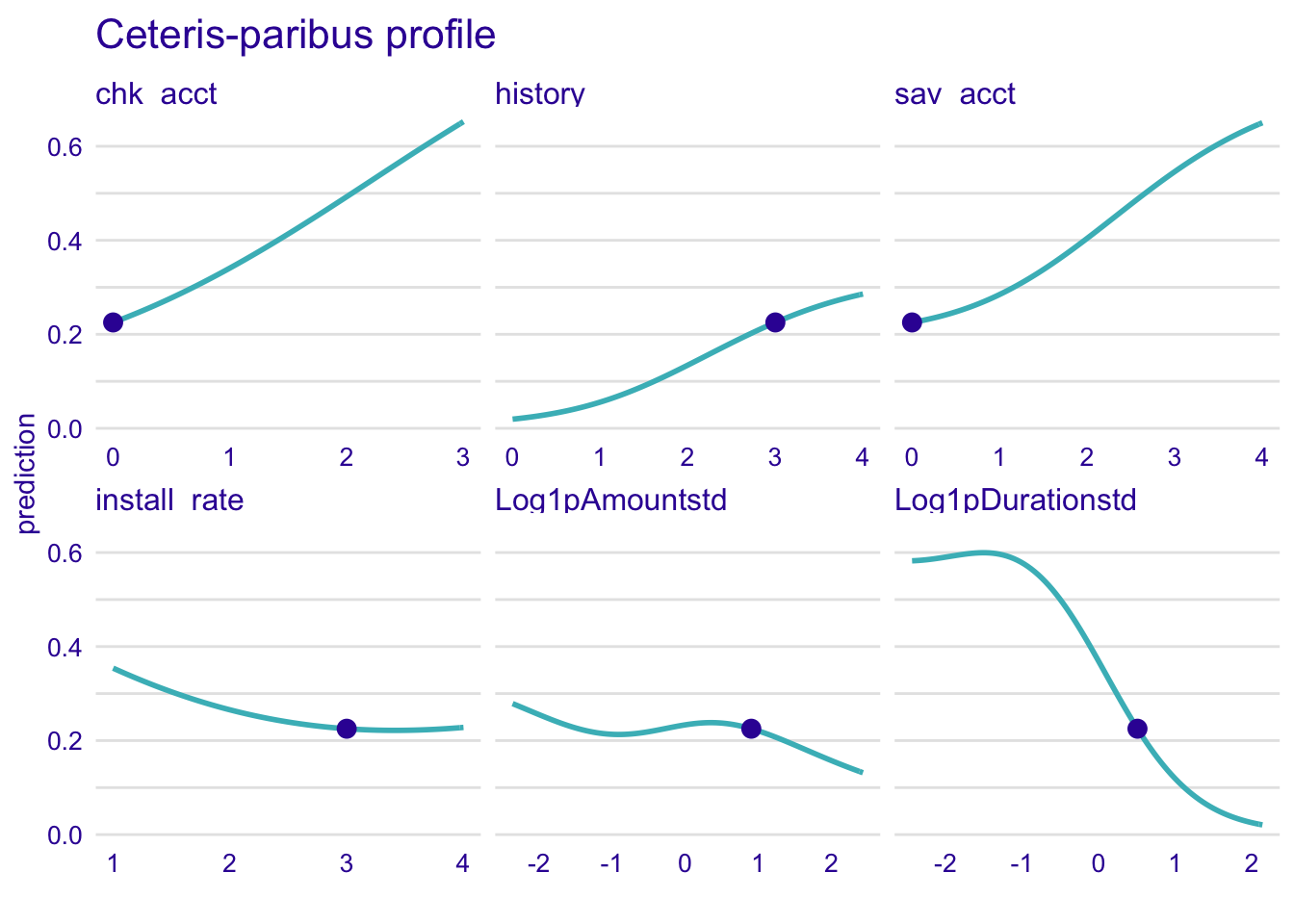
Curves have the shape of a wave, especially for the Log1pDurationstd. It means that the variable predicts a good credit risk between -2 and -1, then the trend is falling.
Common important variables between models
Here, we compare the profiles of the most important common variables in our models.
- chk_acct
- Log1pDurationstd
- sav_acct
- history
#Compare model with common important variables
predict_profile_rf <- predict_profile(explainer_rf, new_observation = single_customer, variables = c("chk_acct", "Log1pDurationstd", "sav_acct", "history"))
predict_profile_glm<- predict_profile(explainer_glm, new_observation = single_customer, variables = c("chk_acct", "Log1pDurationstd", "sav_acct", "history"))
predict_profile_knn <- predict_profile(explainer_knn, new_observation = single_customer, variables = c("chk_acct", "Log1pDurationstd", "sav_acct", "history"))
predict_profile_lda <- predict_profile(explainer_lda, new_observation = single_customer, variables = c("chk_acct", "Log1pDurationstd", "sav_acct", "history"))
predict_profile_nn <- predict_profile(explainer_nn, new_observation = single_customer, variables = c("chk_acct", "Log1pDurationstd", "sav_acct", "history"))

plot(predict_profile_rf, predict_profile_glm, predict_profile_knn, predict_profile_lda, predict_profile_nn, variables = c("chk_acct", "Log1pDurationstd", "sav_acct", "history")) + ggtitle("Ceteris-paribus profile", "")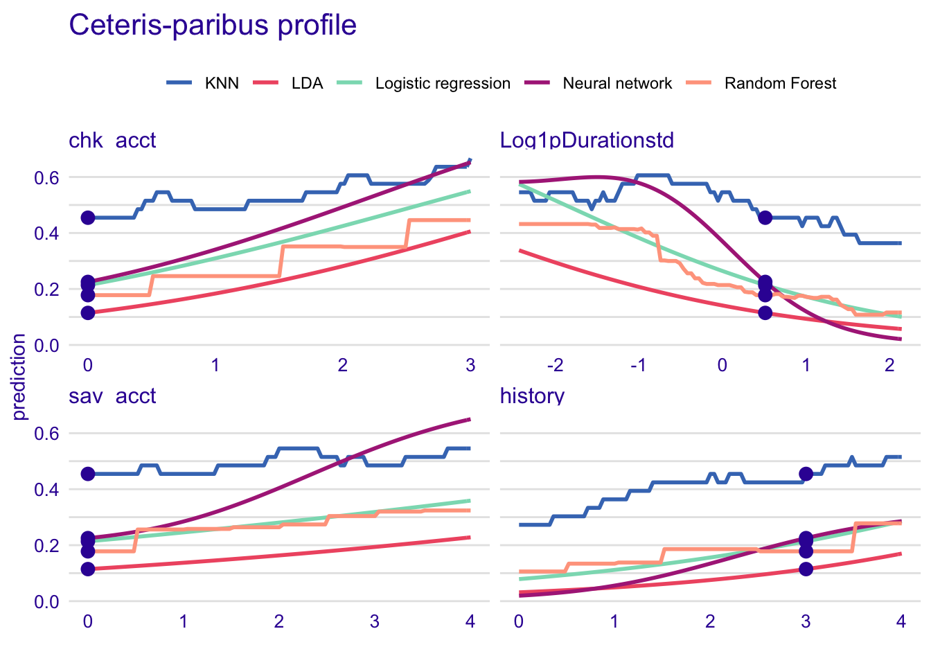
The effect of the variables is overestimated in KNN model. Or, all models besides KNN underestimate the effect in each variable. It can be both reasons.
4.5 Summary of DALEX results
The same important variables emerge in most of our analysed models. We found that the variables chk_acct, Log1pDurationstd and sav_acct play a major role in the predictions and have the same effects in each of our models. These three variables are therefore essential for risk classification. However, we noticed an abnormal trend for the education and history variables. Indeed, the effect of these features does not reflect reality. It is possible that these variables may detract from the results of our models. It would therefore be wise to consider removing them from our prediction models in order to observe the possibility of increasing the predictive capacity of the models.
Finally, in the modeling part, KNN and random forest models had respectively the best accuracy and ROC. However, from this analysis we remarked that those models were not capturing the same effects of the variables. KNN always overestimates the effect of the features compared to the random forest model and reciprocally. Despite the new information provided by this analysis, determining the best model remains tedious. In addition, one should not exclude the naive bayes model which was the best at predicting bad risks.