Chapter 4 Simulation study: Gender and age restrictions

4.1 Gender

library(boot)
library(purrr)

dat_sim <- dat %>%
  nest() %>%
  mutate(area = "Overall") %>%
  bind_rows(dat %>%
              mutate(area = ifelse(area == "0_periurban",
                                   "Periurban",
                                   "Rural")) %>%
              group_by(area) %>%
              nest()) %>%
  crossing(p_out = as.character(unique(dat$nm_sex))) %>%
  mutate(data = map(.x = data, 
                    .f = ~mutate(.x, comm = as.factor(as.character(comm)))),
         boot = map2(.x = data, .y = p_out,
                    .f = ~boot(data = .x,
                               statistic = standardization_bin, 
                               treatment = work_out, 
                               outcome = SEROPOSITIVE, 
                               var_sim = nm_sex,
                               cat_sim = .y,
                               formula1 = f,
                               R = R
                               )),
         p_out_label = ifelse(p_out == "0_female", 
                              "Female", "Male"),
         boot_tab = map2(.x = boot, .y = p_out_label,
                        .f = ~tab_bin(.x, 
                                      cat_sim = .y)))

saveRDS(dat_sim, "./_out/_rds/result_05-sex.rds")

dat_sim_res <- dat_sim %>%
  select(area, p_out_label, boot_tab) %>%
  mutate(p_out_label_s = ifelse(p_out_label == "Female", 
                              "F", "M"),) %>%
  unnest()

4.2 Plots Gender

p_gender <- dat_sim_res %>%
  filter(type != "NE - OBS") %>% #UPDATE
  mutate(type = case_when( #UPDATE
    type == "OBS" ~ "NC",
    type == "FE" ~ "FE",
    type == "NE" ~ "NE",
    type == "FE - NE" ~ "RD [FE - NE]",
    type == "FE - OBS" ~ "RD [FE - NC]")
    ) %>%
  ggplot(aes(x = type, y = mean, col = p_out_label)) +
  geom_hline(aes(yintercept = 0), col = "grey50") +
  geom_rect(aes(xmin = 3.5, xmax = Inf, ymin = -Inf, ymax = Inf), #UPDATE
            alpha = .025, col = NA) +
  geom_linerange(aes(ymin = ll, ymax = ul), alpha = .6, 
                 size = 1.5, 
                 position = position_dodge(width=0.5)) +
  geom_point(size = .7, position = position_dodge(width=0.5)) +
  #guides(col = F) +
  scale_color_npg() +
  scale_x_discrete(limits = c("NC", "FE","NE", 
                              "RD [FE - NE]", "RD [FE - NC]")) +
  #scale_color_viridis_c(option = "B", direction = -1) +
  facet_grid(.~area) +
  #geom_smooth(method = "lm", se = F, size = .2) +
  labs(y = "Standardized mean outcome", x = "",
       col = "Gender") +
  theme_bw() +
  theme(legend.position = "top",
        panel.grid.major.x = element_blank(),
        panel.grid.minor.x = element_blank(),
        axis.text.x = element_text(angle = 90, 
                                   vjust = 0.5, hjust=1))

4.3 Age

library(boot)
library(purrr)

dat <- dat %>%
  mutate(age_bin = ifelse(edad <= 17, "17 and under", 
                          "18 and older"))

dat_sim <- dat %>%
  nest() %>%
  mutate(area = "Overall") %>%
  bind_rows(dat %>%
              mutate(area = ifelse(area == "0_periurban",
                                   "Periurban",
                                   "Rural")) %>%
              group_by(area) %>%
              nest()) %>%
  crossing(p_out = unique(dat$age_bin)) %>%
  mutate(data = map(.x = data, 
                    .f = ~mutate(.x, comm = as.factor(as.character(comm)))),
         boot = map2(.x = data, .y = p_out,
                    .f = ~boot(data = .x,
                               statistic = standardization_bin, 
                               treatment = work_out, 
                               outcome = SEROPOSITIVE, 
                               var_sim = age_bin,
                               cat_sim = .y,
                               formula1 = f,
                               R = R
                               )),
         # p_out_label = ifelse(p_out == "0_female", 
         #                      "Female", "Male"),
         boot_tab = map2(.x = boot, .y = p_out,
                        .f = ~tab_bin(.x, 
                                      cat_sim = .y)))

saveRDS(dat_sim, "./_out/_rds/result_05-age.rds")

dat_sim_res <- dat_sim %>%
  select(area, p_out, boot_tab) %>%
  # mutate(p_out_label_s = ifelse(p_out_label == "Female", 
  #                             "F", "M"),) %>%
  unnest()

4.4 Plots Age

p_age <- dat_sim_res %>%
  filter(type != "NE - OBS") %>% #UPDATE
  mutate(type = case_when( #UPDATE
    type == "OBS" ~ "NC",
    type == "FE" ~ "FE",
    type == "NE" ~ "NE",
    type == "FE - NE" ~ "RD [FE - NE]",
    type == "FE - OBS" ~ "RD [FE - NC]")
    ) %>%
  ggplot(aes(x = type, y = mean, col = p_out)) +
  geom_hline(aes(yintercept = 0), col = "grey50") +
  geom_rect(aes(xmin = 3.5, xmax = Inf, ymin = -Inf, ymax = Inf), #UPDATE
            alpha = .025, col = NA) +
  geom_linerange(aes(ymin = ll, ymax = ul), alpha = .6, 
                 size = 1.5,
                 position = position_dodge(width=0.5)) +
  geom_point(size = .7, position = position_dodge(width=0.5)) +
  #guides(col = F) +
  scale_color_npg() +
  scale_x_discrete(limits = c("NC", "FE","NE", 
                              "RD [FE - NE]", "RD [FE - NC]")) +
  #scale_color_viridis_c(option = "B", direction = -1) +
  facet_grid(.~area) +
  #geom_smooth(method = "lm", se = F, size = .2) +
  labs(y = "Standardized mean outcome", x = "", 
       col = "Age category") +
  theme_bw() +
  theme(legend.position = "top",
        panel.grid.major.x = element_blank(),
        panel.grid.minor.x = element_blank(),
        axis.text.x = element_text(angle = 90, 
                                   vjust = 0.5, hjust=1))

4.5 Summary Plot

library(cowplot)

plot_grid(p_gender, p_age, labels = c("A)", "B)"), ncol = 1)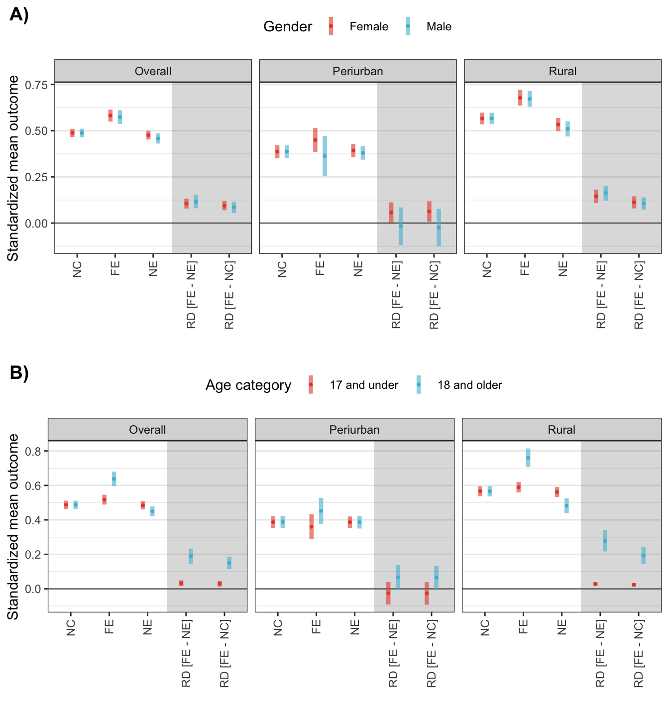

ggsave("./_out/fig5.png", width = 7, height = 7.5,
       dpi = "retina", bg = "white")