Chapter 1 Descriptive Analysis

1.1 Table 1

t1 <- dat %>%
  dplyr::select(area, comm, edad, age_cat, nm_sex, edu_cat,
                work_out, travel_1m,TREATMENT,
                resultado_micro, fever, temp_axilar,
                hist_fever,SEROPOSITIVE)

library(furniture)

t1 %>%
  table1(splitby = ~SEROPOSITIVE, na.rm = F, 
         NAkeep = T, total = T,
         output = "html")

	Total	Negative	Positive
	n = 1790	n = 917	n = 873
area
0_periurban	785 (43.9%)	481 (52.5%)	304 (34.8%)
1_rural	1005 (56.1%)	436 (47.5%)	569 (65.2%)
NA	0 (0%)	0 (0%)	0 (0%)
comm
501_Rumococha	250 (14%)	165 (18%)	85 (9.7%)
502_Santo Tomás	273 (15.3%)	132 (14.4%)	141 (16.2%)
503_Quistococha	262 (14.6%)	184 (20.1%)	78 (8.9%)
901_Gamitanacocha	47 (2.6%)	6 (0.7%)	41 (4.7%)
902_Libertad	179 (10%)	45 (4.9%)	134 (15.3%)
903_Primero de Enero	58 (3.2%)	18 (2%)	40 (4.6%)
904_Salvador	270 (15.1%)	144 (15.7%)	126 (14.4%)
905_Lago Yuracyacu	97 (5.4%)	67 (7.3%)	30 (3.4%)
906_Puerto Alegre	166 (9.3%)	84 (9.2%)	82 (9.4%)
907_Urco Miraño	188 (10.5%)	72 (7.9%)	116 (13.3%)
NA	0 (0%)	0 (0%)	0 (0%)
edad
	29.0 (22.0)	20.6 (18.8)	37.8 (21.8)
age_cat
[0,5]	178 (9.9%)	147 (16%)	31 (3.6%)
(5,15]	568 (31.7%)	405 (44.2%)	163 (18.7%)
(15,30]	299 (16.7%)	148 (16.1%)	151 (17.3%)
(30,50]	388 (21.7%)	126 (13.7%)	262 (30%)
(50,117]	357 (19.9%)	91 (9.9%)	266 (30.5%)
NA	0 (0%)	0 (0%)	0 (0%)
nm_sex
0_female	973 (54.4%)	536 (58.5%)	437 (50.1%)
1_male	817 (45.6%)	381 (41.5%)	436 (49.9%)
NA	0 (0%)	0 (0%)	0 (0%)
edu_cat
Primary or less	1183 (66.1%)	582 (63.5%)	601 (68.8%)
Secondary or Superior	607 (33.9%)	335 (36.5%)	272 (31.2%)
NA	0 (0%)	0 (0%)	0 (0%)
work_out
Inside	1278 (71.4%)	798 (87%)	480 (55%)
Outside	512 (28.6%)	119 (13%)	393 (45%)
NA	0 (0%)	0 (0%)	0 (0%)
travel_1m
No	1436 (80.2%)	794 (86.6%)	642 (73.5%)
Yes	349 (19.5%)	120 (13.1%)	229 (26.2%)
NA	5 (0.3%)	3 (0.3%)	2 (0.2%)
TREATMENT
No treatment	917 (51.2%)	917 (100%)	0 (0%)
Treatment	873 (48.8%)	0 (0%)	873 (100%)
NA	0 (0%)	0 (0%)	0 (0%)
resultado_micro
Negative	1729 (96.6%)	894 (97.5%)	835 (95.6%)
Positive	38 (2.1%)	12 (1.3%)	26 (3%)
NA	23 (1.3%)	11 (1.2%)	12 (1.4%)
fever
No	1764 (98.5%)	900 (98.1%)	864 (99%)
Yes	26 (1.5%)	17 (1.9%)	9 (1%)
NA	0 (0%)	0 (0%)	0 (0%)
temp_axilar
	36.2 (0.5)	36.2 (0.5)	36.2 (0.5)
hist_fever
No	1572 (87.8%)	821 (89.5%)	751 (86%)
Yes	218 (12.2%)	96 (10.5%)	122 (14%)
NA	0 (0%)	0 (0%)	0 (0%)
SEROPOSITIVE
Negative	917 (51.2%)	917 (100%)	0 (0%)
Positive	873 (48.8%)	0 (0%)	873 (100%)
NA	0 (0%)	0 (0%)	0 (0%)

t1 %>%
  table1(splitby = ~area, na.rm = F, 
         NAkeep = T, total = T,
         output = "html")

	Total	0_periurban	1_rural
	n = 1790	n = 785	n = 1005
area
0_periurban	785 (43.9%)	785 (100%)	0 (0%)
1_rural	1005 (56.1%)	0 (0%)	1005 (100%)
NA	0 (0%)	0 (0%)	0 (0%)
comm
501_Rumococha	250 (14%)	250 (31.8%)	0 (0%)
502_Santo Tomás	273 (15.3%)	273 (34.8%)	0 (0%)
503_Quistococha	262 (14.6%)	262 (33.4%)	0 (0%)
901_Gamitanacocha	47 (2.6%)	0 (0%)	47 (4.7%)
902_Libertad	179 (10%)	0 (0%)	179 (17.8%)
903_Primero de Enero	58 (3.2%)	0 (0%)	58 (5.8%)
904_Salvador	270 (15.1%)	0 (0%)	270 (26.9%)
905_Lago Yuracyacu	97 (5.4%)	0 (0%)	97 (9.7%)
906_Puerto Alegre	166 (9.3%)	0 (0%)	166 (16.5%)
907_Urco Miraño	188 (10.5%)	0 (0%)	188 (18.7%)
NA	0 (0%)	0 (0%)	0 (0%)
edad
	29.0 (22.0)	30.6 (21.8)	27.7 (22.2)
age_cat
[0,5]	178 (9.9%)	52 (6.6%)	126 (12.5%)
(5,15]	568 (31.7%)	227 (28.9%)	341 (33.9%)
(15,30]	299 (16.7%)	169 (21.5%)	130 (12.9%)
(30,50]	388 (21.7%)	176 (22.4%)	212 (21.1%)
(50,117]	357 (19.9%)	161 (20.5%)	196 (19.5%)
NA	0 (0%)	0 (0%)	0 (0%)
nm_sex
0_female	973 (54.4%)	461 (58.7%)	512 (50.9%)
1_male	817 (45.6%)	324 (41.3%)	493 (49.1%)
NA	0 (0%)	0 (0%)	0 (0%)
edu_cat
Primary or less	1183 (66.1%)	427 (54.4%)	756 (75.2%)
Secondary or Superior	607 (33.9%)	358 (45.6%)	249 (24.8%)
NA	0 (0%)	0 (0%)	0 (0%)
work_out
Inside	1278 (71.4%)	688 (87.6%)	590 (58.7%)
Outside	512 (28.6%)	97 (12.4%)	415 (41.3%)
NA	0 (0%)	0 (0%)	0 (0%)
travel_1m
No	1436 (80.2%)	768 (97.8%)	668 (66.5%)
Yes	349 (19.5%)	17 (2.2%)	332 (33%)
NA	5 (0.3%)	0 (0%)	5 (0.5%)
TREATMENT
No treatment	917 (51.2%)	481 (61.3%)	436 (43.4%)
Treatment	873 (48.8%)	304 (38.7%)	569 (56.6%)
NA	0 (0%)	0 (0%)	0 (0%)
resultado_micro
Negative	1729 (96.6%)	742 (94.5%)	987 (98.2%)
Positive	38 (2.1%)	20 (2.5%)	18 (1.8%)
NA	23 (1.3%)	23 (2.9%)	0 (0%)
fever
No	1764 (98.5%)	771 (98.2%)	993 (98.8%)
Yes	26 (1.5%)	14 (1.8%)	12 (1.2%)
NA	0 (0%)	0 (0%)	0 (0%)
temp_axilar
	36.2 (0.5)	36.2 (0.5)	36.1 (0.5)
hist_fever
No	1572 (87.8%)	719 (91.6%)	853 (84.9%)
Yes	218 (12.2%)	66 (8.4%)	152 (15.1%)
NA	0 (0%)	0 (0%)	0 (0%)
SEROPOSITIVE
Negative	917 (51.2%)	481 (61.3%)	436 (43.4%)
Positive	873 (48.8%)	304 (38.7%)	569 (56.6%)
NA	0 (0%)	0 (0%)	0 (0%)

1.2 Descriptives

1.3 Proportions

library(tidyverse)
library(ggmosaic)
library(innovar)

prop_bar <- function(cat_var, title = NULL, l.pos = "none", labx = "") {
  
  title1 <- if (is.null(title)) {expression(cat_var)} else {title}
  
  var1 <- enquo(cat_var)
  
  t1 %>%
  filter(!is.na(resultado_micro)) %>%
  mutate(area = ifelse(area == "0_periurban", "Periurban", "Rural"),
         nm_sex = ifelse(nm_sex == "0_female", "Female", "Male"),
         var2 = !!var1,
         mm = ifelse(resultado_micro=="Positive", "micro+", "micro-"),
         ss = ifelse(SEROPOSITIVE=="Positive", "sero+", "sero-"),
         out = paste0(mm, " | ",ss),
         age_cat = factor(age_cat),
         out = factor(out),
         out = fct_rev(out)) %>%
    filter(!is.na(var2)) %>%
  
  ggplot() +
  geom_mosaic(aes(x = product(out, age_cat), fill = out)#, 
                  #offset = 0.1
                  ) +
    scale_fill_innova(palette = "mlobo") +
  # scale_fill_discrete_sequential(palette="Heat 2",
  #                                rev = F) +
    # scale_fill_manual(values=c("#1b4332", "#b7e4c7", 
    #                            "#006d77", "#83c5be")) +
  labs(y = "proportion", fill = "Outcome", x = labx) +
  theme_minimal() +
  facet_grid(~var2) +
  ggtitle(title1) +
  theme(panel.grid.major = element_blank(),
        panel.grid.minor = element_blank(),
        axis.text.y=element_blank(),
        axis.ticks.y=element_blank(),
        axis.text.x = element_text(angle = 90, vjust = 0.5, hjust=1),
        legend.position = l.pos)

  
}

f1a <- prop_bar(area, "Area")
f1b <- prop_bar(nm_sex, "Sex")
f1c <- prop_bar(work_out, "Activities outside village")
f1d <- prop_bar(travel_1m, "Travel in the last month")
f1e <- prop_bar(edu_cat, "Education", labx = "Age category")
f1f <- prop_bar(hist_fever, "Fever in last week", labx = "Age category")

library(cowplot)

legend <- get_legend(
  prop_bar(hist_fever, "Fever in last week", "bottom") +
    theme(legend.box.margin = margin(0, 0, 0, 12))
)

lplot <- plot_grid(legend)

plots <- plot_grid(f1a, f1b, f1c, f1d, f1e, f1f, ncol = 2)

p2 <- plot_grid(plots, lplot, ncol = 1, rel_heights = c(9,1))
p2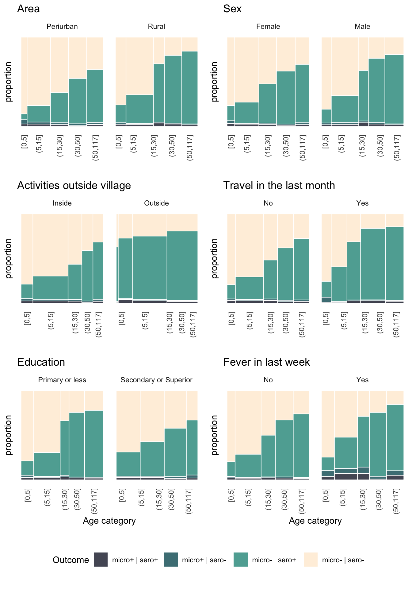

1.4 Maps

1.4.1 Static

library(maptools)
library(ggspatial)

# library(ggmap)
# map <- get_map(location = st_bbox(d2) %>% as.numeric(), maptype = "watercolor", source = "osm", zoom = 10)
# 
# ggmap(map) + 
#   coord_sf(crs = st_crs(3857)) +
#   geom_sf(data = d2 %>%
#             group_by(id_house) %>%
#             summarise(p = mean(sero)), 
#           aes(col = p), inherit.aes = FALSE, alpha=.4) +
#   scale_color_viridis(option = "magma") +
#   labs(col = "Household \nSeropositivity Rate")


library(basemaps)

# get_maptypes()

set_defaults(map_service = "carto",
             map_type = "light_no_labels")

# basemap_ggplot(d2)

data1 = d2 %>%
            group_by(id_house) %>%
            summarise(p = mean(sero)) %>%
  st_transform(crs = 3857)


buffer <- st_bbox(d2) %>%
  st_as_sfc() %>%
  st_buffer(10000)

p1 <- ggplot() +
  basemap_gglayer(buffer) +
  coord_sf(expand = F) +
  scale_fill_identity() +
  geom_sf(data = data1, aes(col = p)) +
  coord_sf(expand = F) +
  labs(col = "Household \nSeropositivity rate") +
  scale_color_viridis_c(option = "magma") + 
  annotation_scale(location = "br") +
  coord_sf(expand = F) +
  annotation_north_arrow(location = "tl",
                         style = north_arrow_nautical) +
  coord_sf(expand = F) +
  #theme_void() + 
  theme(panel.background = element_rect(fill = "white", 
                                        colour = "black"),
        legend.position = "bottom") +
  guides(colour = guide_colourbar(title.position="top", 
                                  title.hjust = 0.5),
         size = guide_legend(title.position="top", 
                             title.hjust = 0.5))

## Loading basemap 'light_no_labels' from map service 'carto'...

plot_grid(p1, p2, nrow = 1, labels = c("A)", "B)"),
          rel_widths = c(4,5))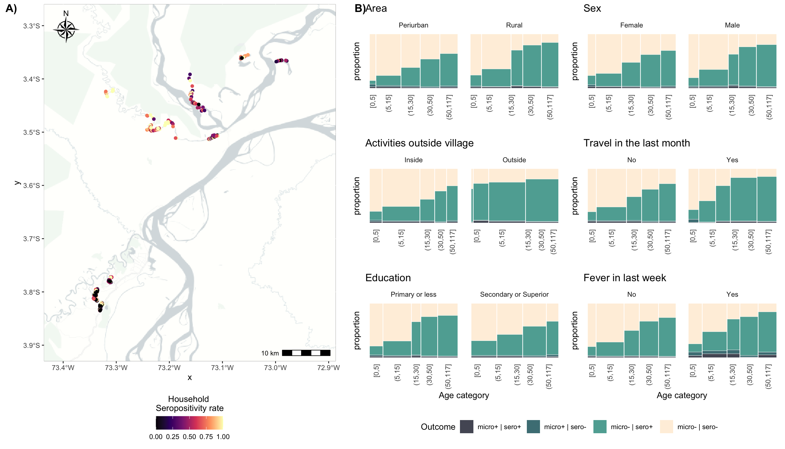

ggsave("./_out/fig1.png", width = 14, height = 8,
       dpi = "retina", bg = "white")

1.4.2 Dynamic

library(leaflet)

dat_ci_map <- d2 %>%
  group_by(id_house) %>%
  summarise(p = mean(sero, na.rm = T), area = first(area), age = mean(edad, na.rm = T)) %>%
  filter(!is.na(p)) %>%
  filter(!is.infinite(p)) %>%
  dplyr::mutate(lat = sf::st_coordinates(.)[,2],
                long = sf::st_coordinates(.)[,1])

pal <- colorBin("inferno", bins = seq(0,1,.1), reverse=T) 

dat_ci_map %>%
  leaflet() %>%
  addTiles() %>%
  addCircles(lng = ~long, lat = ~lat, color = ~ pal(p),
             popup = paste("ID Household", dat_ci_map$id_house, "<br>",
                           "Area:", dat_ci_map$area, "<br>",
                           "Mean age:", dat_ci_map$age, "<br>",
                           "Prevalence:", dat_ci_map$p)) %>%
  addLegend("bottomright",
            pal = pal, values = ~p,
            title = "Prevalence") %>%
  addScaleBar(position = c("bottomleft"))