Chapter 4 IPTW 4
4.1 Data
rm(list = ls())
library(tidyverse)
library(kableExtra)
library(jtools)
library(sf)
load("./_data/rscd_jr.RData")

dat <- d2 %>%
  dplyr::select(id_house, comm, id_study:viaje_ult_mes,SEROPOSITIVE, main_act_ec:fumigacion, area) %>%
  st_set_geometry(NULL) %>%
  mutate(viaje_ult_mes = ifelse(viaje_ult_mes=="9999", NA, viaje_ult_mes),
         viaje_ult_mes = factor(ifelse(viaje_ult_mes=="2", "1_yes", "0_no")),
         SEROPOSITIVE = ifelse(SEROPOSITIVE=="Positive",1,0),
         work_out = factor(ifelse(as.numeric(main_act_ec)>0 & as.numeric(main_act_ec)<6, "outside", "inside"))) %>% filter(complete.cases(.))

dat_gf_1 <- dat %>%
  #dplyr::select(viaje_ult_mes, work_out, edad, SEROPOSITIVE, nm_sex, comm, area) %>%
  mutate(id = seq(1:n()),
         time = 0,
         viaje_ult_mes = as.integer(as.numeric(viaje_ult_mes)-1),
         work_out = as.numeric(work_out)-1,
         sex_male = as.numeric(nm_sex)-1,
         SEROPOSITIVE = as.integer(SEROPOSITIVE),
         edad = as.numeric(edad)#,
         #edad = edad*edad
         ) %>%
  filter(complete.cases(.)) %>%
  as.data.frame()
4.2 The product method
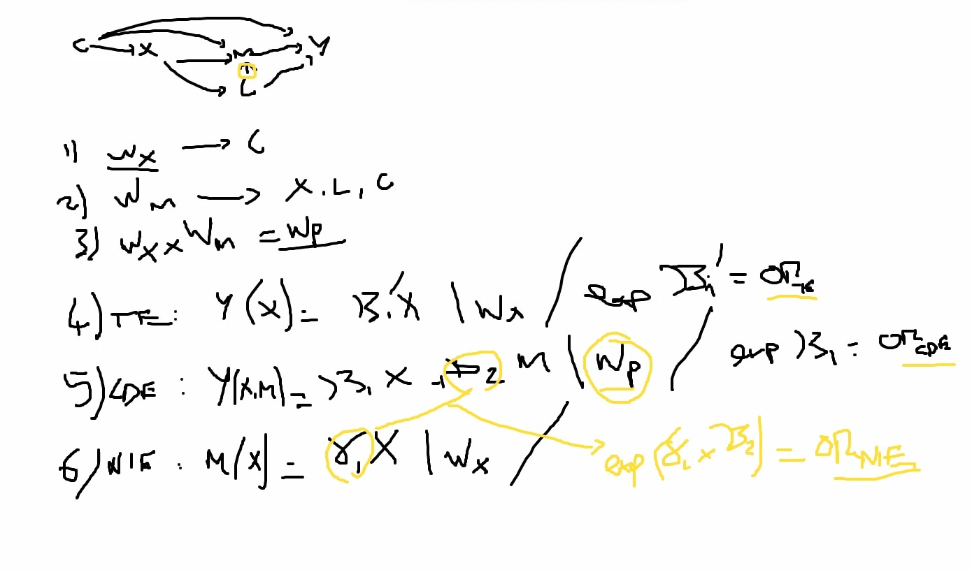
4.3 Weights
#C = edad
#X = sex_male
#M = work_out
#L = viaje_ult_mes
#Y = SEROPOSITIVE

#p1 <- glm(sex_male ~ ... , data = dat_gf, family = "binomial")
dat_gf_2 <- dat_gf_1 %>%
  mutate(wx = 1) #%>%
  # mutate(ps1 = predict(p1, type = "response"),
  #        wx = ifelse(sex_male==1, 1/ps1, 1/(1-ps1)))
p <- glm(work_out ~ 1, data = dat_gf_2, family = "binomial")

p2 <- glm(work_out ~ (sex_male + edad + fumigacion + animales_casa + factor(tipo_casa))^2,
          data = dat_gf_2, family = "binomial")

dat_gf <- dat_gf_2 %>%
  mutate(p = predict(p, type="response"),
         ps2 = predict(p2, type = "response"),
         wm = ifelse(work_out==1, p/ps2, p/(1-ps2)),
         wp = wm*wx)

dat_gf %>%
  ggplot(aes(x=ps2, fill= factor(work_out))) +
  geom_density(alpha=.5) +
  #scale_x_continuous(trans = "log10") +
  theme_nice() +
  theme(legend.position = "top")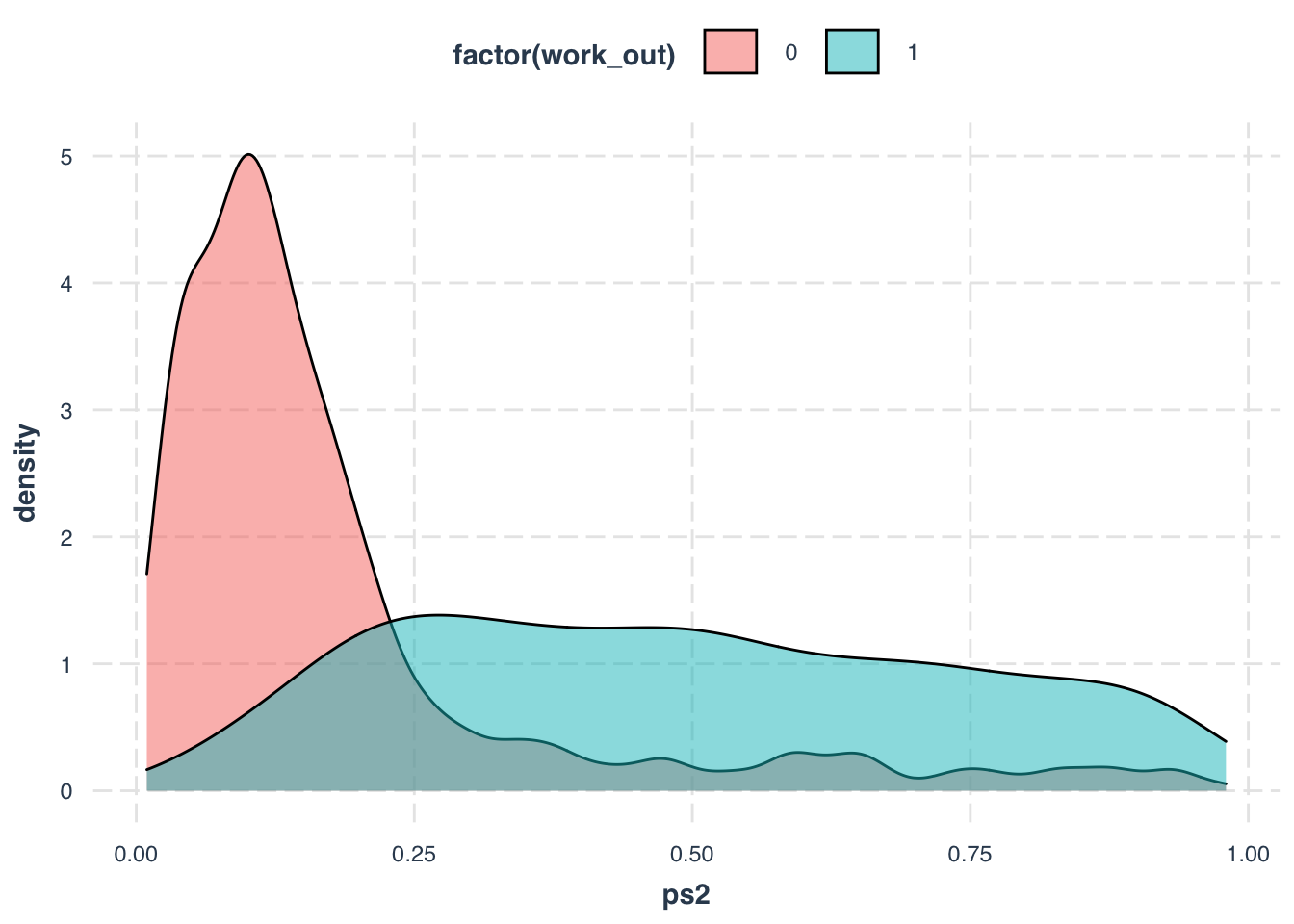
4.4 Mediation
# Total Effect
te <- glm(SEROPOSITIVE ~ sex_male + comm, data = dat_gf, weights = wx, family = "binomial")
(te.t <- summ(te, confint = T))| Observations | 1773 |
| Dependent variable | SEROPOSITIVE |
| Type | Generalized linear model |
| Family | binomial |
| Link | logit |
| 𝛘²(10) | 186.51 |
| Pseudo-R² (Cragg-Uhler) | 0.13 |
| Pseudo-R² (McFadden) | 0.08 |
| AIC | 2292.14 |
| BIC | 2352.43 |
| Est. | 2.5% | 97.5% | z val. | p | |
|---|---|---|---|---|---|
| (Intercept) | -0.80 | -1.07 | -0.52 | -5.63 | 0.00 |
| sex_male | 0.30 | 0.11 | 0.50 | 3.01 | 0.00 |
| comm502 | 0.74 | 0.38 | 1.09 | 4.07 | 0.00 |
| comm503 | -0.19 | -0.56 | 0.19 | -0.97 | 0.33 |
| comm901 | 2.60 | 1.70 | 3.49 | 5.68 | 0.00 |
| comm902 | 1.75 | 1.31 | 2.18 | 7.94 | 0.00 |
| comm903 | 1.36 | 0.74 | 1.98 | 4.28 | 0.00 |
| comm904 | 0.52 | 0.16 | 0.87 | 2.85 | 0.00 |
| comm905 | -0.17 | -0.67 | 0.34 | -0.65 | 0.52 |
| comm906 | 0.64 | 0.23 | 1.04 | 3.06 | 0.00 |
| comm907 | 1.13 | 0.74 | 1.53 | 5.61 | 0.00 |
| Standard errors: MLE |
(te.e <- te.t$coeftable[2,1])## [1] 0.3031542# Controlled Direct Effect
cde <- glm(SEROPOSITIVE ~ sex_male + work_out + comm, data = dat_gf, weights = wp, family = "binomial")
(cde.t <- summ(cde, confint = T))| Observations | 1773 |
| Dependent variable | SEROPOSITIVE |
| Type | Generalized linear model |
| Family | binomial |
| Link | logit |
| 𝛘²(11) | 212.39 |
| Pseudo-R² (Cragg-Uhler) | 0.20 |
| Pseudo-R² (McFadden) | 0.18 |
| AIC | 596.18 |
| BIC | 661.94 |
| Est. | 2.5% | 97.5% | z val. | p | |
|---|---|---|---|---|---|
| (Intercept) | -1.11 | -1.58 | -0.65 | -4.69 | 0.00 |
| sex_male | 0.44 | 0.14 | 0.74 | 2.88 | 0.00 |
| work_out | 1.30 | 0.95 | 1.66 | 7.22 | 0.00 |
| comm502 | 1.57 | 1.01 | 2.12 | 5.55 | 0.00 |
| comm503 | -0.01 | -0.59 | 0.58 | -0.02 | 0.99 |
| comm901 | 3.03 | 1.42 | 4.64 | 3.69 | 0.00 |
| comm902 | 2.03 | 1.33 | 2.74 | 5.65 | 0.00 |
| comm903 | 1.13 | 0.19 | 2.08 | 2.35 | 0.02 |
| comm904 | 0.45 | -0.12 | 1.01 | 1.55 | 0.12 |
| comm905 | -0.68 | -1.45 | 0.10 | -1.72 | 0.09 |
| comm906 | 0.37 | -0.25 | 0.99 | 1.18 | 0.24 |
| comm907 | 1.43 | 0.80 | 2.06 | 4.43 | 0.00 |
| Standard errors: MLE |
(cde.e <- cde.t$coeftable[2,1])## [1] 0.4408013(b2 <- cde.t$coeftable[3,1])## [1] 1.302777# Natual Indirect Effect
nie <- glm(work_out ~ sex_male + comm, data = dat_gf, weights = wx, family = "binomial")
(nie.t <- summ(nie, confint = T))| Observations | 1773 |
| Dependent variable | work_out |
| Type | Generalized linear model |
| Family | binomial |
| Link | logit |
| 𝛘²(10) | 334.09 |
| Pseudo-R² (Cragg-Uhler) | 0.25 |
| Pseudo-R² (McFadden) | 0.16 |
| AIC | 1746.71 |
| BIC | 1807.00 |
| Est. | 2.5% | 97.5% | z val. | p | |
|---|---|---|---|---|---|
| (Intercept) | -2.89 | -3.37 | -2.41 | -11.77 | 0.00 |
| sex_male | 0.86 | 0.63 | 1.09 | 7.27 | 0.00 |
| comm502 | 0.79 | 0.22 | 1.36 | 2.73 | 0.01 |
| comm503 | -0.99 | -1.84 | -0.15 | -2.31 | 0.02 |
| comm901 | 2.21 | 1.46 | 2.96 | 5.77 | 0.00 |
| comm902 | 2.16 | 1.61 | 2.71 | 7.67 | 0.00 |
| comm903 | 1.93 | 1.21 | 2.65 | 5.24 | 0.00 |
| comm904 | 2.04 | 1.51 | 2.56 | 7.62 | 0.00 |
| comm905 | 2.12 | 1.50 | 2.74 | 6.72 | 0.00 |
| comm906 | 2.32 | 1.76 | 2.88 | 8.12 | 0.00 |
| comm907 | 1.82 | 1.26 | 2.37 | 6.43 | 0.00 |
| Standard errors: MLE |
(a1 <- nie.t$coeftable[2,1])## [1] 0.8616512(nie.e <- a1*b2) ## [1] 1.122539# TE
cde.e + nie.e## [1] 1.56334te.e## [1] 0.3031542# PROPORTION MEDIATED
(exp(cde.e)*(exp(nie.e)-1))/((exp(cde.e)*exp(nie.e))-1)## [1] 0.85324784.5 4-way decompositon
4.5.1 Hand calculation
4.5.1.1 outcome regression
eq1 <- glm(SEROPOSITIVE ~ sex_male*work_out + comm, weights = wp, data = dat_gf, family = "binomial")
(summ.eq1 <- summ(eq1, confint = T))| Observations | 1773 |
| Dependent variable | SEROPOSITIVE |
| Type | Generalized linear model |
| Family | binomial |
| Link | logit |
| 𝛘²(12) | 212.75 |
| Pseudo-R² (Cragg-Uhler) | 0.20 |
| Pseudo-R² (McFadden) | 0.17 |
| AIC | 599.06 |
| BIC | 670.31 |
| Est. | 2.5% | 97.5% | z val. | p | |
|---|---|---|---|---|---|
| (Intercept) | -1.09 | -1.56 | -0.61 | -4.50 | 0.00 |
| sex_male | 0.38 | 0.01 | 0.74 | 2.01 | 0.04 |
| work_out | 1.22 | 0.77 | 1.67 | 5.34 | 0.00 |
| comm502 | 1.57 | 1.02 | 2.13 | 5.56 | 0.00 |
| comm503 | 0.00 | -0.58 | 0.59 | 0.02 | 0.99 |
| comm901 | 3.02 | 1.41 | 4.63 | 3.68 | 0.00 |
| comm902 | 2.04 | 1.33 | 2.74 | 5.67 | 0.00 |
| comm903 | 1.14 | 0.20 | 2.08 | 2.37 | 0.02 |
| comm904 | 0.45 | -0.11 | 1.02 | 1.57 | 0.12 |
| comm905 | -0.68 | -1.46 | 0.10 | -1.71 | 0.09 |
| comm906 | 0.38 | -0.24 | 1.01 | 1.21 | 0.22 |
| comm907 | 1.44 | 0.81 | 2.08 | 4.46 | 0.00 |
| sex_male:work_out | 0.19 | -0.44 | 0.83 | 0.59 | 0.55 |
| Standard errors: MLE |
(O1 <- summ.eq1$coeftable[2,1])## [1] 0.3764244(O2 <- summ.eq1$coeftable[3,1])## [1] 1.219127(O3 <- summ.eq1$coeftable[4,1])## [1] 1.5727654.5.1.2 mediator regression
eq2 <- glm(work_out ~ sex_male + comm, data = dat_gf, weights = wx, family = "binomial")
(summ.eq2 <- summ(eq2, confint = T))| Observations | 1773 |
| Dependent variable | work_out |
| Type | Generalized linear model |
| Family | binomial |
| Link | logit |
| 𝛘²(10) | 334.09 |
| Pseudo-R² (Cragg-Uhler) | 0.25 |
| Pseudo-R² (McFadden) | 0.16 |
| AIC | 1746.71 |
| BIC | 1807.00 |
| Est. | 2.5% | 97.5% | z val. | p | |
|---|---|---|---|---|---|
| (Intercept) | -2.89 | -3.37 | -2.41 | -11.77 | 0.00 |
| sex_male | 0.86 | 0.63 | 1.09 | 7.27 | 0.00 |
| comm502 | 0.79 | 0.22 | 1.36 | 2.73 | 0.01 |
| comm503 | -0.99 | -1.84 | -0.15 | -2.31 | 0.02 |
| comm901 | 2.21 | 1.46 | 2.96 | 5.77 | 0.00 |
| comm902 | 2.16 | 1.61 | 2.71 | 7.67 | 0.00 |
| comm903 | 1.93 | 1.21 | 2.65 | 5.24 | 0.00 |
| comm904 | 2.04 | 1.51 | 2.56 | 7.62 | 0.00 |
| comm905 | 2.12 | 1.50 | 2.74 | 6.72 | 0.00 |
| comm906 | 2.32 | 1.76 | 2.88 | 8.12 | 0.00 |
| comm907 | 1.82 | 1.26 | 2.37 | 6.43 | 0.00 |
| Standard errors: MLE |
(B0 <- summ.eq2$coeftable[1,1])## [1] -2.88827(B1 <- summ.eq2$coeftable[2,1])## [1] 0.8616512(B2 <- summ.eq2$coeftable[3,1])## [1] 0.7892644(B3 <- summ.eq2$coeftable[4,1])## [1] -0.9939624(B4 <- summ.eq2$coeftable[5,1])## [1] 2.209652(B5 <- summ.eq2$coeftable[6,1])## [1] 2.160096(B6 <- summ.eq2$coeftable[7,1])## [1] 1.929365(B7 <- summ.eq2$coeftable[8,1])## [1] 2.036803(B8 <- summ.eq2$coeftable[9,1])## [1] 2.117415(B9 <- summ.eq2$coeftable[10,1])## [1] 2.320721(B10 <- summ.eq2$coeftable[11,1])## [1] 1.8172734.5.1.3 Summary
- Do we need to include non-significant betas?? (mediator regression)
(CDE <- O1)## [1] 0.3764244(INTref <- O3*(B0+B2+B3+B4+B5+B6+B7+B8+B9+B10))## [1] 18.08422(INTmed <- O3*B1)## [1] 1.355175(PIE <- O2*B1)## [1] 1.050462(TE <- CDE + INTref + INTmed + PIE)## [1] 20.86628CDE/TE## [1] 0.01803984INTref/TE## [1] 0.8666719INTmed/TE## [1] 0.0649457PIE/TE## [1] 0.05034259(TIE <- PIE + INTmed)## [1] 2.405638(PDE <- CDE + INTref)## [1] 18.46064(TDE <- CDE +INTref + INTmed)## [1] 19.81582(PE <- PIE + INTref +INTmed)## [1] 20.48985(PAI <- INTref + INTmed)## [1] 19.439394.5.2 Package
#-----------------------------------------------------------------------------------------------------------
# All libraries here
library(boot)
library(survival)
library(data.table)
library(foreign)
library(dummies)
#library(GenABEL)
#library(dummies)
#-----------------------------------------------------------------------------------------------------------
# Sources import here

# this script should be run from the same folder where src.R is
source('./4way-decomposition-master/src.R')
#-----------------------------------------------------------------------------------------------------------
# Define your parameters here!!!

#Path to save results
output<-"./Test_results.csv"

#Define variables
A<<-'sex_male'
M<<-'work_out'
Y<<-'SEROPOSITIVE'
COVAR<<-c('comm_502', 'comm_503', 'comm_901', 'comm_902', 'comm_903', 'comm_904', 'comm_905', 'comm_906',
          'comm_907')

#1=binary 0=continuous
outcome=1
mediator=1

#Assign levels for the exposure that are being compared;
#for mstar it is the level at which to compute the CDE and the remainder of the decomposition
a<<-1
astar<<-0
mstar<<-0

#Boostrap number of iterations
N_r=5

#-----------------------------------------------------------------------------------------------------------
####### DONT TOUCH FROM HERE #######
#------------------------------------------------------------------------------------------------------------

# Reading data file
#data<-read.spss(data_path, to.data.frame=T) #TODO spss/csv/txt (?)
data<-dat_gf %>%
  mutate(area = as.numeric(area)) %>%
  fastDummies::dummy_cols(remove_first_dummy = TRUE)

if (! prod(c(A,Y,M,COVAR) %in% names(data) ) )  {stop('Some of defined variable names are not in data file!')}

if ( mediator==1 & outcome==1 ) {  save_results(output=output, boot_function=boot.bMbO, N=N_r)  }
if ( mediator==0 & outcome==1 ) {  save_results(output=output, boot_function=boot.cMbO, N=N_r)  }
if ( mediator==1 & outcome==0 ) {  save_results(output=output, boot_function=boot.bMcO, N=N_r)  }
if ( mediator==0 & outcome==0 ) {  save_results(output=output, boot_function=boot.cMcO, N=N_r)  }


table.4wd <- read.csv("./Test_results.csv")
kable(table.4wd)| X | Estimand | Estimate | LCL | UCL |
|---|---|---|---|---|
| 1 | Total Effect Risk Ratio | 2.0489677 | 2.1423445 | 2.4808605 |
| 2 | Total Excess Relative Risk | 1.0489677 | 1.1423445 | 1.4808605 |
| 3 | Excess Relative Risk due to CDE | 0.3384432 | 0.2081473 | 0.4649223 |
| 4 | Excess Relative Risk due to INTref | 0.2326412 | 0.2901057 | 0.5882195 |
| 5 | Excess Relative Risk due to INTmed | 0.2258876 | 0.2657566 | 0.5988550 |
| 6 | Excess Relative Risk due to PIE | 0.2519957 | 0.0856387 | 0.3061863 |
| 7 | Proportion CDE | 0.3226441 | -0.1143264 | 0.3844542 |
| 8 | Proportion INTref | 0.2217811 | 0.2279973 | 0.6427878 |
| 9 | Proportion INTmed | 0.2153427 | 0.2017792 | 0.6690355 |
| 10 | Proportion PIE | 0.2402321 | -0.1974968 | 0.2021998 |
| 11 | Overall Proportion Mediated | 0.4555748 | 0.3875484 | 0.5310306 |
| 12 | Overall Proportion Attributable to Interaction | 0.4371238 | 0.4297765 | 1.3118232 |
| 13 | Overall Proportion Eliminated | 0.6773559 | 0.6155458 | 1.1143264 |